Excel Magic Trick 1104: Add with 6 Criteria (AND and OR Criteria) with Criteria/Data Mismatch

Get free Excel 2010 Slaying Excel Dragon's DVD with 53 videos!
First 25 to watch, comment and Like this interview video AND subscribe to ExcelTV:
EXCEL TV - Episode 07 with Mike "ExcelIsFun" Girvin
46:49 min shows original formula example
Video link below video!!!

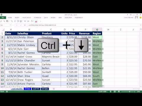
See how to add unit numbers with AND and OR Criteria where the criteria are given as years and months but date column contains serial number dates. See how to use SUMIFS function to do both AND and OR Criteria:
1. (01:20 min) Set up of problem with criteria and data mismatch.
2. (02:37 min) Use LOOKUP Function & Big Number lookup_value concept to lookup last number.
3. (02:37 min) Create a formula element that will have a duel relative and absolute cell reference when criteria is not listed in each row.
4. (04:50 min) Use MONTH function and text month name concatenated with number to trick MONTH to deliver a month number.
5. (05:41 min) Use DATE, LOOKUP and MONTH function to create serial number date for the first of each month given text date formula inputs.
6. (06:10 min) Use EOMONTH, DATE, LOOKUP and Month to to create serial number date for the end of each month given text date formula inputs.
7. (07:30 min) Create Defined Names From Selection with a keyboard: Ctrl + F3.
8. (08:00 min) Use SUMIFS with 6 total criteria: 3 AND Criteria and 3 OR Criteria. See how to use SUMIFS with a function argument array operation to enact OR Criteria for adding.
9. (11:40 min) See how SUMPRODUCT can add the resultant array of items created by an array formula element without using Ctrl + Shift + Enter

Lots of cool keyboard shortcuts in this video.

[excelisfun]

Excel Magic Trick 1104: Add with 6 Criteria (AND and OR Criteria) with Criteria & Data Mismatch 
Get free Excel 2010 Slaying Excel Dragon's DVD with 53 videos!
First 25 to watch, comment and Like this interview video AND subscribe to ExcelTV:
EXCEL TV - Episode 07 with Mike "ExcelIsFun" Girvin
EXCEL TV - Episode 07 with Mike "ExcelIsFun" Girvin
 <<< 46:49 min shows original formula example
Video link below video!!!

[Exceltvshowseries]

Thank you so much for your ongoing support of our channel.  You are a ROCK STAR, Mike Girvin.

[TGUGCL]

Thank you for putting so much details in the description Of the video! It makes it easy to find what you are looking. Also, thank you for giving references to earlier videos.

[carlplz]

Exellent video, very instructive... Thank you

[IjeomaMbelu]

You are an excel god! !! Thank you for all the tips...really helpful

[BillSzysz]

Very cool!!  So many tricks in one formula :)))
Thanks, Mike :))

[TickyMN]

Wow, amazing how you piece formulas together.

[roeunkhloy]

Love the videos, books, and examples.

[oberghaus]

Mike your tricks are awesome. Thanks for sharing.

[MBVDJ_service]

Thanks you really make me look good :) love the knowledge

[LHpitcher]

Hope I got a dvd! Love your stuff ExcelIsFun! Your videos help me out immensely, so thank you for making these informative vids!

[christopherdulce]

I am using this formula to get the cells with values. =if(E$8="", G7, E$8)

[jmof]

You're like the Neo from the Matrix of Excel.

[sohelahmed]

Sir, I try to watch all your trick. I am a great fan of your Ctrl+Shift+Enter Array Formula.

[ahmedasu]

Amazing presentation
let me get the dvd plz

[VSP]

Dear Mike, I appreciate so much what you are doing. I see that your creativity in using Excel is so big and I am surprised each time you create such formulas as that of today. As a silly question, if we have a data format day/month/year, as we do in some countries, will be a change in the formula?? I guess YES but I do not know how. The implication will be that we have something like this 1/1/2014, 1/02/2014 

[emirhantekin]

We could have just done it with Pivot Table, am i right?

[XLarium]

Hello Mike
I would suggest to enter the missing years (E9, E10, E12, E13) and the formula will be simpler:
{=SUM((TEXT(Date, "JJJJMMM")=$E8&$F8)*(Units)*(Sales_Rep=TRANSPOSE(G$5:G$7)))}

[krn]

Seen some of this one before.. What number am I?  

[BillSzysz]

Very cool!!  So many tricks in one formula :)))
Thanks, Mike :)))