filmov
tv
Euler's formula: A cool proof

Показать описание
numbers and it satisfies i^2=-1. This famous formula has been around for hundreds of
years and it was first proved by Euler in the 1740s using power series. You write cosine as a
power series, sin as a power series, the exponential as a power series and then you equate real
and imaginary parts. In this presentation I am going to do something a little bit different I
am going to use an approach that is related to differential equations. And it is based on the fact
that solutions to certain initial value problems involving ordinary differential equations the
solutions are unique. Euler did the
power series method and there is a Khan academy video about that as well there is also
a limit way to prove it which you will find on Wikipedia and there is also a way that Gil Strang
does it using calculus and assuming that this can be written in the r cis θ form. Well let me show you and one of the
nice things about the method that I am going to show you is that you can prove all sorts of other
identities with the method just by using some basic differential equations. The proof for this result I am just going to
motivate it by a mathematician called Richard Bellman so certainly the proof I am going to
show you would be known but you just do not see it very many places. I am going
to let a function be this e^i*x. I am going to differentiate this function and see what
differential equation f satisfies. So if I differentiate just by treating i as a constant
bring the i to the front now if I differentiate again okay so i would come to the front and we know
that i^2=-1 so I will get the following. Notice that f'' is the negative of f. Now I
have got a differential equation 00:00-04:20.
If I plug in say x=0 I will get e to the 0 which is e^0 which is 1 and if I go up here and
plug in x=0 I will get i*e^0 which is just i. Now we have an initial value problem okay in
particular this is a linear second order problem with constant coefficients and we have some
initial conditions associated with it. Okay this IVP or initial value problem has a unique solution
and that is you would learn that say in a first course in ordinary differential equations. Now
because the coefficients are constant in this problem it is actually easy to solve this problem for
f.
You can look at the characteristic equation the characteristic equation would be
something like r^2+1 =0 and so the roots will be complex and you can write the general
solution to this problem as a linear combination of cosine and sines where the a and b, because
of the initial conditions, could be complex numbers. If you put in x=0 instead x=1, differentiate said
x=0 and equate it with i then you will get these two values for a and b okay. So If I go up to here
and plug in a=1, b=i I will get the following. 04:20-07:53.
We have shown that e^(i*x) satisfies a certain initial value problem and then we
have taken that initial value problem and we solved it. Now because the initial value problem
under consideration is a special initial value problem it has special properties because of the
uniqueness there is one and only one solution to that problem. The two functions that we have
started with or derived here, the f and the g, must be equal. Okay so by uniqueness of solutions to our IVP or our
initial value problem this and this must be the same. So f must be identically equal to g, that
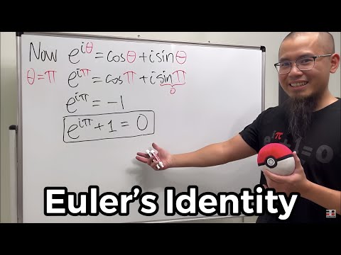
what these sort of 3 horizontal lines mean. That is e^(i*x) must equal cos(x) +i*sin(x). 07:53-09:39.
Alright so there are some advantages and disadvantages of this proof. You need to
know a little bit about differential equations to really appreciate the style of proof that I have
mentioned. One of the positives as far as I can see for the method of proof that I have just
shown you is that it gives you a nice way of applying the idea of uniqueness of solutions to
differential equations and initial value problems. You can use the theory of differential
equations to prove all sorts of nice formulae or identities. Now is it as simple as
say Euler's method using power series well no okay no. But i still think it is really nice to talk
about this proof because I have not seen it anywhere I do not think it is on youtube. I have seen
a first order type approach to prove this identity but I have never seen second order approach
okay so I think I am sort of adding something new there alright. Now if you get a chance see
what other identities you can prove involving trig functions using differential equations. There is a
whole bunch of them you can prove and it provides a nice alternative than say a geometric
approach.
years and it was first proved by Euler in the 1740s using power series. You write cosine as a
power series, sin as a power series, the exponential as a power series and then you equate real
and imaginary parts. In this presentation I am going to do something a little bit different I
am going to use an approach that is related to differential equations. And it is based on the fact
that solutions to certain initial value problems involving ordinary differential equations the
solutions are unique. Euler did the
power series method and there is a Khan academy video about that as well there is also
a limit way to prove it which you will find on Wikipedia and there is also a way that Gil Strang
does it using calculus and assuming that this can be written in the r cis θ form. Well let me show you and one of the
nice things about the method that I am going to show you is that you can prove all sorts of other
identities with the method just by using some basic differential equations. The proof for this result I am just going to
motivate it by a mathematician called Richard Bellman so certainly the proof I am going to
show you would be known but you just do not see it very many places. I am going
to let a function be this e^i*x. I am going to differentiate this function and see what
differential equation f satisfies. So if I differentiate just by treating i as a constant
bring the i to the front now if I differentiate again okay so i would come to the front and we know
that i^2=-1 so I will get the following. Notice that f'' is the negative of f. Now I
have got a differential equation 00:00-04:20.
If I plug in say x=0 I will get e to the 0 which is e^0 which is 1 and if I go up here and
plug in x=0 I will get i*e^0 which is just i. Now we have an initial value problem okay in
particular this is a linear second order problem with constant coefficients and we have some
initial conditions associated with it. Okay this IVP or initial value problem has a unique solution
and that is you would learn that say in a first course in ordinary differential equations. Now
because the coefficients are constant in this problem it is actually easy to solve this problem for
f.
You can look at the characteristic equation the characteristic equation would be
something like r^2+1 =0 and so the roots will be complex and you can write the general
solution to this problem as a linear combination of cosine and sines where the a and b, because
of the initial conditions, could be complex numbers. If you put in x=0 instead x=1, differentiate said
x=0 and equate it with i then you will get these two values for a and b okay. So If I go up to here
and plug in a=1, b=i I will get the following. 04:20-07:53.
We have shown that e^(i*x) satisfies a certain initial value problem and then we
have taken that initial value problem and we solved it. Now because the initial value problem
under consideration is a special initial value problem it has special properties because of the
uniqueness there is one and only one solution to that problem. The two functions that we have
started with or derived here, the f and the g, must be equal. Okay so by uniqueness of solutions to our IVP or our
initial value problem this and this must be the same. So f must be identically equal to g, that
what these sort of 3 horizontal lines mean. That is e^(i*x) must equal cos(x) +i*sin(x). 07:53-09:39.
Alright so there are some advantages and disadvantages of this proof. You need to
know a little bit about differential equations to really appreciate the style of proof that I have
mentioned. One of the positives as far as I can see for the method of proof that I have just
shown you is that it gives you a nice way of applying the idea of uniqueness of solutions to
differential equations and initial value problems. You can use the theory of differential
equations to prove all sorts of nice formulae or identities. Now is it as simple as
say Euler's method using power series well no okay no. But i still think it is really nice to talk
about this proof because I have not seen it anywhere I do not think it is on youtube. I have seen
a first order type approach to prove this identity but I have never seen second order approach
okay so I think I am sort of adding something new there alright. Now if you get a chance see
what other identities you can prove involving trig functions using differential equations. There is a
whole bunch of them you can prove and it provides a nice alternative than say a geometric
approach.
 0:11:56
Euler's formula: A cool proof
 0:00:33
The Euler's formula explained!
 0:07:27
Euler's Formula and Graph Duality
 0:26:57
The most beautiful equation in math, explained visually [Euler’s Formula]
 0:03:57
Proof of Euler's Formula Without Taylor Series
 0:00:56
Euler's Formula Proof
 0:00:39
A nice approach to Euler's formula
 0:01:00
How Euler's formula works
 0:13:50
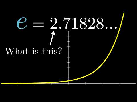
What's so special about Euler's number e? | Chapter 5, Essence of calculus
 0:03:50
The Most Beautiful Equation in Math
 0:07:19
Euler’s identity proof for calculus 2 students!
 0:00:29
The proof for Euler's famous identity! #shorts #maths #calculus #education
 0:00:20
The Euler Formula
 0:08:42
Eulers formula
 0:51:16
What is Euler's formula actually saying? | Ep. 4 Lockdown live math
 0:00:57
Euler's identity
 0:07:36
Proof of Euler's Formula
 0:00:21
Hardest formula in the World!!! Euler's formula...
 0:15:55
Proof: Euler's Formula for Plane Graphs | Graph Theory
 0:00:34
Proof of Euler’s Formula 👨🏼🏫📝
 0:13:11
Why do trig functions appear in Euler's formula?
 0:06:56
Euler's Formula & Euler's Identity - Proof via Taylor Series
 0:10:58
Euler`s Formula in Graph Theory proof | Discrete Mathematics | Ganitya
 0:00:12
A Golden Version Of Euler’s Identity
Комментарии