filmov
tv
Excel Row Numbering: Number The Visible Rows - Episode 2328
Показать описание
Microsoft Excel Tutorial: Number the visible rows.
Welcome to the MrExcel Netcast, where we bring you the best tips and tricks for mastering Excel. In today's episode, we will be discussing how to number only the visible rows in your data set. This is a common issue faced by many Excel users, and we have the perfect solution for you.
Our question for today comes from Jennifer in Daytona, who wants to filter her data to show only her best-selling product, tomatoes. She then wants to number just the visible rows and leave the rest with a dash. However, the usual method of using the fill handle does not work when there is a filter applied. So, what's the solution?
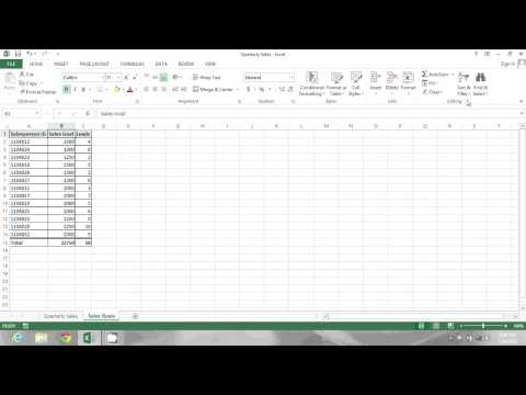
After some brainstorming, we came up with a simple yet effective solution. We will count the numbers above the visible rows and add one to each row. This will give us a sequential numbering for the visible rows, and we can easily fill the rest with dashes. To do this, we use the COUNTIF function and an expanding range. This trick will save you time and effort, and you can use it for any filtered data set.
But what if you want to number all the rows, including the hidden ones? We have a solution for that too. By using the COUNTIF function and an expanding range, we can get a mix of numbers for all the rows. And the best part is, when you filter the data, the numbers will adjust accordingly. This is a handy trick for organizing your data and making it easier to work with.
If you enjoyed this tip, make sure to hit the subscribe button and ring the bell icon to stay updated with our latest videos. Also, don't forget to check out my new book, MrExcel 2020: Seeing Excel Clearly, for more useful tips and tricks. And if you have any questions or comments, feel free to leave them down below in the comments section. Thank you for watching, and I'll see you in the next netcast from MrExcel.
Jennifer from Daytona wants to Filter a data set to only show Tomato and then number the visible rows. But you can't do this with the Fill Handle. In today's episode, a couple of formulas to solve the problem.
This video answers these common search terms:
how to count only visible cells in excel
how to count pnlyu visible cells in excell
how to count only visible rows in excel
how to count visible rows in excel
how to only count visible cells in excel
how to number only visible cells in excel
how to number pnlyu visible cells in excell
how to number only visible rows in excel
how to number visible rows in excel
how to only number visible cells in excel
how to count a filtered column in excel
how to count only filtered cells in excel
how to count in excel when filtering
how to count rows in excel when filtered
how to count in filtered excel table
how to count filter in excel
how to count with filter in excel
how to do count rows that are filtered in excel
can excell count rows with filters
how to put a count filter in excell
#excel
#microsoft
#exceltutorial
#microsoftexcel
#excelformula
#excelformulasandfunctions
Table of Contents
(0:00) Problem Statement: Number the Visible Rows
(0:32) Filter by Selection & Fill Handle Does not work
(0:45) COUNT all numbers above plus one
(1:21) Choose Go To Special Blanks
(1:40) Enter a dash with apostrophe minus minus
(1:58) Method 2: COUNTIF all rows above
(2:23) When you filter, the matches are numbered
(2:39) Clicking Like really helps the algorithm
Welcome to the MrExcel Netcast, where we bring you the best tips and tricks for mastering Excel. In today's episode, we will be discussing how to number only the visible rows in your data set. This is a common issue faced by many Excel users, and we have the perfect solution for you.
Our question for today comes from Jennifer in Daytona, who wants to filter her data to show only her best-selling product, tomatoes. She then wants to number just the visible rows and leave the rest with a dash. However, the usual method of using the fill handle does not work when there is a filter applied. So, what's the solution?
After some brainstorming, we came up with a simple yet effective solution. We will count the numbers above the visible rows and add one to each row. This will give us a sequential numbering for the visible rows, and we can easily fill the rest with dashes. To do this, we use the COUNTIF function and an expanding range. This trick will save you time and effort, and you can use it for any filtered data set.
But what if you want to number all the rows, including the hidden ones? We have a solution for that too. By using the COUNTIF function and an expanding range, we can get a mix of numbers for all the rows. And the best part is, when you filter the data, the numbers will adjust accordingly. This is a handy trick for organizing your data and making it easier to work with.
If you enjoyed this tip, make sure to hit the subscribe button and ring the bell icon to stay updated with our latest videos. Also, don't forget to check out my new book, MrExcel 2020: Seeing Excel Clearly, for more useful tips and tricks. And if you have any questions or comments, feel free to leave them down below in the comments section. Thank you for watching, and I'll see you in the next netcast from MrExcel.
Jennifer from Daytona wants to Filter a data set to only show Tomato and then number the visible rows. But you can't do this with the Fill Handle. In today's episode, a couple of formulas to solve the problem.
This video answers these common search terms:
how to count only visible cells in excel
how to count pnlyu visible cells in excell
how to count only visible rows in excel
how to count visible rows in excel
how to only count visible cells in excel
how to number only visible cells in excel
how to number pnlyu visible cells in excell
how to number only visible rows in excel
how to number visible rows in excel
how to only number visible cells in excel
how to count a filtered column in excel
how to count only filtered cells in excel
how to count in excel when filtering
how to count rows in excel when filtered
how to count in filtered excel table
how to count filter in excel
how to count with filter in excel
how to do count rows that are filtered in excel
can excell count rows with filters
how to put a count filter in excell
#excel
#microsoft
#exceltutorial
#microsoftexcel
#excelformula
#excelformulasandfunctions
Table of Contents
(0:00) Problem Statement: Number the Visible Rows
(0:32) Filter by Selection & Fill Handle Does not work
(0:45) COUNT all numbers above plus one
(1:21) Choose Go To Special Blanks
(1:40) Enter a dash with apostrophe minus minus
(1:58) Method 2: COUNTIF all rows above
(2:23) When you filter, the matches are numbered
(2:39) Clicking Like really helps the algorithm
 0:02:37
How to Automate Row numbers in Excel?
 0:02:41
How to Number Rows in Excel (The Simplest Way)
 0:01:04
How to automatically number rows in Microsoft Excel
 0:00:26
Excel Sort Column by Numbers in Ascending/Descending Order (2020)
 0:04:09
Do NOT Drag Down to Create Numbered Lists in Excel! Here's Why.
 0:03:55
Sequential Numbering in Excel with the ROW function by Chris Menard
 0:10:09
How to Automatically Add Numbers in Rows in Excel | Serial Auto-Numbering in Excel after Row Insert
 0:01:02
Microsoft Excel Rows and Columns Labeled As Numbers in Microsoft Excel Tutorial
 1:05:07
Excel Hour - Learn to Excel with the FP&A Guy
 0:04:11
How to Insert Serial Number Automatically in Excel
 0:09:48
4 Ways To Create Numbered Lists In Excel - Dynamic And Professional
 0:02:54
Excel Tips - Quickly Fill Series of Numbers in a Few Seconds Fill Command
 0:15:02
7 Quick & Easy Ways to Number Rows in Excel
 0:00:59
How To Fill Numbers In Excel Quickly And Easily!
 0:01:02
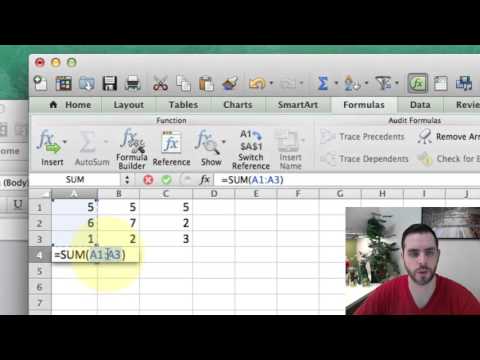
How to Sum a Column or Row of Excel Cells
 0:04:57
How to put sequence number in excel or Google Sheet Automatically
 0:07:41
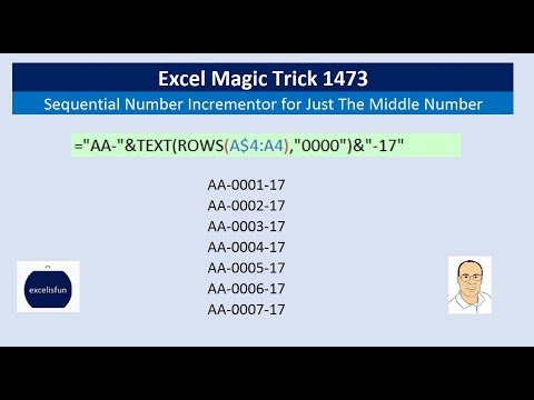
Excel Magic Trick 1473: Sequential Number Incrementor for Just The Middle Number: AA-0009-17
 0:00:37
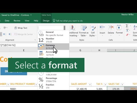
Format numbers in cells in Microsoft Excel
 0:04:01
Clean Mobile Numbers list using Len and Right functions in Excel
 0:04:23
Excel Formula to Increment Numbers: 1-6, 7-12, 13-18 for Raffle Ticket - Excel Magic Trick 1585
 0:03:12
How to Count Rows in Excel | Counting Rows in Excel sheet
 0:01:35
How to Sort Ascending Numerically in Excel : MS Excel Tips
 0:09:51
SEQUENCE function in Excel | Formula for returning a sequence of numbers | Excel Off The Grid
 0:02:40
Excel not formatting cell contents as numbers, won't sum cells -decimal separator - comma and p...
Комментарии