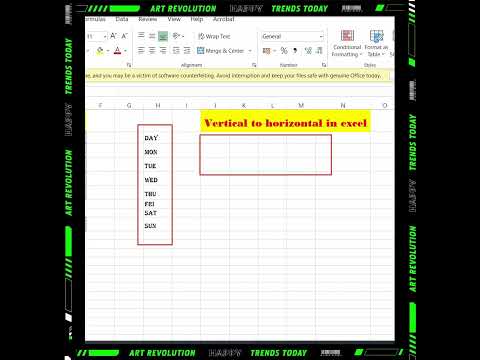
3 Ways to Transpose Excel Data (Rotate data from Vertical to Horizontal or Vice Versa)

Discover three effective methods to transpose your data in Excel. Whether you're looking for a static solution or a dynamic approach, this tutorial covers all bases. Learn the traditional copy-paste method, the TRANSPOSE function, and a unique formula trick for rotating your data effortlessly.

✨ Key Highlights:
▪️ Static Method - Copy and Paste as Transpose: Explore the simplest way to transpose data using the Paste Special feature, ideal for one-time data reorganization.
▪️ Dynamic Method - TRANSPOSE Function: Dive into the TRANSPOSE function, an array formula that dynamically updates your data. Understand how to select the result area and use Ctrl+Shift+Enter to activate the formula.
▪️ Simple Formula Trick for Transposing: Learn a clever method to transpose data using a text-based approach, followed by a quick find-and-replace action to convert text into formulas.

Check out 3 ways to Transpose your data in Excel. These are useful when you want to switch the orientation of your data from columns to rows or vice versa. I show you how to:

00:00 Switch Data from Rows to Columns in Excel - or Vice Versa
00:25 Static approach - copy and paste as transpose
00:54 Use the Transpose Function to Rotate Data
02:54 Use a Simple Formula Trick to Transpose

Note: Once you get dynamic arrays, writing the Transpose function becomes super simple. You no longer need to highlight the result area first, nor press control + shift + enter.

★ Links to related videos:

🚩Let’s connect on social:

Note: This description contains affiliate links, which means at no additional cost to you, we will receive a small commission if you make a purchase using the links. This helps support the channel and allows us to continue to make videos like this. Thank you for your support!

#excel

[rajaaslam]

Hi Leila,
Your 3rd method is so outside the box thinking.
I love it.
Thanks so much.

[robertlohman]

I came up with this formula: =INDIRECT("B"&COLUMN()) and copy across. Bob Umlas showed your example #3 in one of his books (This isn't Excel, it's magic). Method #3 is definitely the easiest.

[theshivelyfamily]

Method 3 is so genius and yet so simple. Perfect.

[excelisfun]

Yes indeed, Method Three : ) Ctrl + H Rules! Thanks for the vid, Teammate!

[debojyotiojha]

You make my day with the third version. I am enthralled both with your beauty and excel art 😎😎

[movetomarco]

I can't believe how quickly you helped me including finding you in the search. I've been using Excel for probably longer than you've been alive (1987). I've stuck with a very old version and finally was forced to upgrade. I used to teach Excel but now need to have you teach me.

[nonoobott]

OMG! You're just amazing Leila. And of course, the 3rd method for me is slick. You're the real MVP!

[KirkNeddy]

Method 1 is the reason I came here. For me it's the fastest because when I'm needing this I'm usually just looking for a quick static representation. I use method 2 when needing dynamic, although 3 is fun! Also love the info about dynamic arrays!

[kapcons]

Leila is one of the Trainers whose position is in TOP 99th Percentile!! It’s always pleasure to watch her teaching with different style and perspective. Hatsoff !

[ThalassaMavri]

Method 3 is the best. Thank you Leila, great tip! I was doing it in a static mode, and it was driving me crazy!

[mloebab]

This is the first time I like tutorial videos...thank you Leila....a good combination of intelligence, knowledge and public speaking will keep you moving forward

[turboconch]

Method 3 is what I needed after I spent 3 hours trying to figure this out!!! Amazing work!!

[anishpillai]

Method 3 was a smart way to do it. I use method 1 mostly because I never had to link with the original table. I have also used offset function but I don't remember the formula. It basically would offset rows as we copy to the right. Thanks for the video.

[OzduSoleilDATA]

NICE! Very nice. I like that lg-replacement move.

[opknox]

Method 3 saved my neck! Thank you for the tutorial, Leila. I had 30, 000 values to put into 22 columns in a specific order. After doing the first two rows, I was able to drag it down to the last needed row. BIG time saver!

[GWShark]

Whoever figured out method 3 deserves a monument :) BTW in case you have not noticed, do the replacement of the prefix by = AFTER you dragged and filled ALL cells you'll need. Once you replace it you won't be able to drag and fill anymore and get the right values

[John-urjn]

As always, your help is much appreciated. This was a very helpful lesson.

[Aesthetic]

Love your teaching style! Simply put yet so effective. Appreciate the tutorials (:

[Pablo_]

Working since last 4 years in excel never knoew the 3rd method exist.
Amazing !!!❤

[rebecab.]

That's actually saving my report.... works perfectly! Thank you so much!