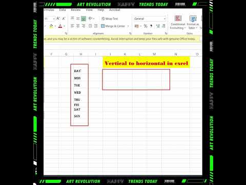
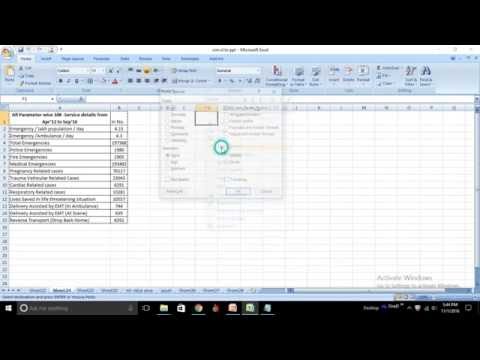
How to Change HORIZONTAL Data to VERTICAL in Excel (NO Transpose Function needed)

Struggling with transposing data in Excel? Discover a clever hack to transform horizontal data into a vertical format efficiently!

🔍 What's Inside:
▪️ Revamped Hack: Explore an advanced method for transposing data, overcoming the limitations of traditional techniques.
▪️ Step-by-Step Guide: Follow a clear, detailed walkthrough to transpose your data with ease.
▪️ Bob Umlas' Method: Learn a unique approach using the R1C1 reference style for seamless data manipulation.

In this Excel tutorial, we explore an efficient hack for transposing data from a horizontal row to a vertical column. If you previously encountered challenges with manual and time-consuming methods, this technique will simplify the process.

Another option is to use the Excel TRANSPOSE function. One thing I don't like about the Transpose formula is that it's an array function and you need to remember to press Control shift enter (at least until you get dynamic array functionality). You also need to highlight the answer area first before inputting the Transpose formula.

🚩Let’s connect on social:

Note: This description contains affiliate links, which means at no additional cost to you, we will receive a small commission if you make a purchase using the links. This helps support the channel and allows us to continue to make videos like this. Thank you for your support!

#excel

[lynton]

Leila, not only are you an outstanding teacher but you made a point of thanking Bob for his contribution. It would have been easier for you to do this video without mentioning him. That you did mention him, elevates you to the highest level of great teachers.Thank you.

[imfjthc]

Leila you are amazing!!! I spent entire night to manually write it down each sell reference with an equal sign. This makes my life easy. I appreciate it a lot.

[wayneedmondson]

Hi Leila. Thanks for the new video. In viewing it, I remembered my post to your original video with my method #4 as follows (using your worksheet visible in the video as the example):
1. In cell A4, make a formula reference as: =A$2; in cell A5, make a formula reference as: = A$3
2. Copy the contents of A4:A5 to the right through M4:M5 (or further if you want to pad for future additions to the source data)
3. Highlight A4:M5 and press CTRL+C
4. Move the pointer to cell D7 and press CTRL+ALT+V, click on the Transpose checkbox and press enter; use the format painter to copy the format of A2 or A3 to D7:E7
5. The previously horizontal orientation will now be vertical and the cell formulas will reference back to your original horizontal data (i.e. will be linked to the original data)
6. Delete the helper formulas in A4:M5
I find the above a pretty quick hack to go from horizontal to vertical (lock the rows in the interim step) and from vertical to horizontal (lock the columns in the interim step) and with the bonus that the transposed cells are linked back to the source. As in your method, you can copy beyond the current range of data and format to hide the zeros, if you want to have more linked cells for future additions to the source.
So, that is my tip for this challenge. I hope you and any others find if useful when needing to transpose source data to the opposite orientation while maintaining a formula link back to the source. Thumbs up!
PS - Just read below the OFFSET methods from Bondi and Pawan.. those are GOLD.. even faster than my method #4 hack! Learn something new and valuable every day on your channel!

[BondiMacF]

I haven't seen that one yet. Very good. I'd always been frustrated that letters won't drag down. I suppose you could use =char(65) to get an A, and to drag it down you can do =char(row(a65)).


My favoured method for transposing however would be =OFFSET($A$1, COLUMN(A1), ROW(A1))


That way if you add a new row of data below your horizontal table you just drag your formula accross on your transposed output table or you can drag your formula down if you add new data to the right of your data table.

[pwnyadav]

Great video...There is a super hack of transposing:
=Offset($A$2, column(A1)-1, row(A1)-1)

[georgetosounidis]

Oh my god (or should I say “goddess “?).
That was simply mind blowing!!!

[BannuIlmiBethak]

it was very helpful thank you very much

[nonsoamamchukwu]

Good one, Leila! I must be so lucky to find this on time! Thanks

[amirnetherlands]

Always the quickest and best solutions.

[sachinrv]

Thanks Leila and Bob; wonderful video; R1C1 is an amazing trick and very easy to follow for anyone. Love you guys, Cheers !

[gautamsarkar]

Thank you Leila, have been an ardent fan of your channel and it has helped me solved many problems helping me improve my Excel skills

[anv.]

Thank you Leila. Your tricks are amazing. Glad to learn them.

[sumitgoyal]

I want to say deeply thank you ☺.... I use your method today in office.... I was so excited that it really work perfectly 😊.... A very informative video for me... I am feeling to say thanks to you once again 😊

[francisconava]

I love your lessons miss. Greetings from México

[ExcelFormulasHacks]

I didn't came across a situation where I can use this. But this is awesome . But I knew this can be done by this method when I saw the data in your video. 🙂

[SenthilvelMurugesan]

I would wish to give a love for the hacks and tricks

[katerina]

Thank you so much Leila, I like so much your tricks in making excel so efficient and easy, always great to think out of the box

[chelseawarren]

Oh my gosh, this is such a lifesaver! Thank you 💛💛💛 ^Chelsea

[luisquismondo]

My favorite: =OFFSET(Sheet1!$B$2, COLUMN(A1)-1, ROW(A1)-1)

[excelisfun]

Great Video!!! I just wish when Microsoft introduced the R1C1 references back in their first version, that it had stuck and we used then today too (becasue they are easier to understand than the A1 references...)