filmov
tv
How to Compare Two Columns in Excel For Matches & Differences Using Formula
Показать описание
How to Compare Two Columns in Excel For Matches & Differences Using Formula
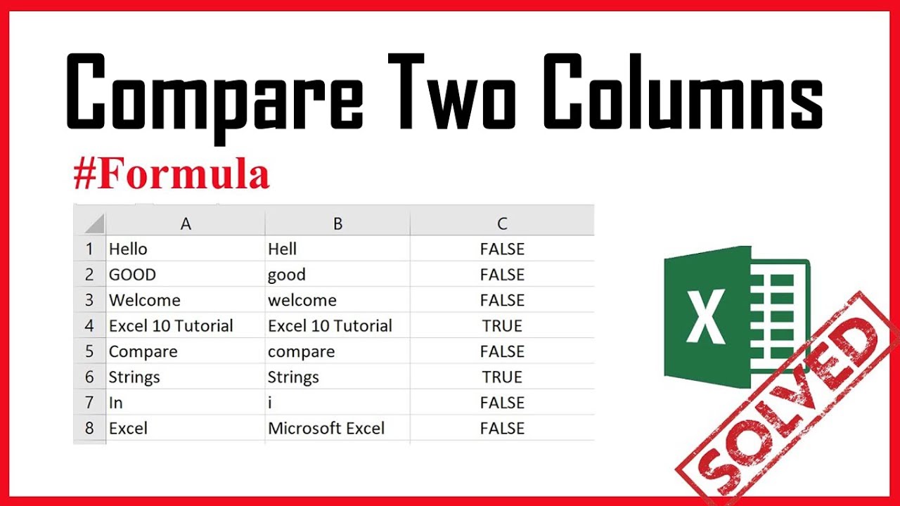
In this excel tutorial, I'll show you how you can compare two columns in excel for matches & differences using Formula based on the strings or value.
There are several ways you can compare two columns in excel, but using the exact Function in excel is the easiest them all. We'll also be able to use this technique to compare two lists to find out if they are an exact match or not. It will also allow us to see if they are case sensitive or not.
Let's learn how to compare two columns based on values. I'm going to show you two Formula to compare two cells or columns. Let's go for the first one:
=EXACT(A1, B1)
The Function above is the use of Exact Function. By this Function, Excel will compare cell A1 & B1 to figure out if they are an exact match. It will also look for case sensitivity. If the cell A1 has a value in All uppercase and if the cell B1 has the same value all in lowercase, it will say false because the case didn't match. So, using this Formula, we can tell excel to compare two columns for matches or Differences. This is a great way to compare 2 columns in excel
Now, the second Formula is a simple one.
=A1=B1
This Formula will make the same comparison except for case sensitivity. For example: If the cell A1 has a value in All uppercase and if the cell B1 has the same value all in lowercase, it will say TRUE because the case doesn't matter here. It just focuses on the text strings. So, you can use this Formula to compare text strings in excel.
So, this is how you can compare two columns excel. These two are the easiest and effective ways for column comparison in excel. Thanks for reading.
#Formula #Compare #Columns
Thanks for watching.
-------------------------------------------------------------------------------------------------------------
Support the channel with as low as $5
-------------------------------------------------------------------------------------------------------------
Please subscribe to #excel10tutorial
Playlists:
Social media:
 0:06:16
Compare Two Columns in Excel to Find Differences or Similarities
 0:03:18
How to Compare Two Columns in Excel to Find Differences (The Easiest Way)
 0:06:17
Compare Two Columns in Excel (for Matches & Differences)
 0:01:43
How to highlight values that appear in two columns | Compare Two Columns in Excel for Matches
 0:04:49
Excel How To Compare Two Columns (3 ways) | Excel Formula Hacks
 0:04:02
Excel : How to Compare Two Columns
 0:02:23
How to Compare Two Columns in Excel For Matches & Differences Using Formula
 0:00:30
Use The And Function Compare Two Columns in Excel #nkexcelclasses #excel #short
 2:04:56
DL24T3 W3 Full Pass of ANN
 0:07:16
Compare Two Lists and Find Matches & Differences with 1 Formula - Excel Magic Trick
 0:14:45
HOW TO: compare two columns in Excel using VLOOKUP
 0:03:45
Excel: Compare two columns using Vlookup
 0:04:35
EXCEL: How to compare two columns and highlight common values
 0:02:57
Compare Two Columns in Excel (for Matches & Differences)
 0:05:31
Compare Two Columns with Microsoft Excel Power Query | Excel Formula Hacks
 0:00:55
How To Compare Two Columns And Delete Matches In Excel?
 0:01:29
Compare Two Columns And Return Values From The Third Column
 0:00:59
Compare two lists to find missing values using VLOOKUP in Excel - Excel Tips and Tricks
 0:00:39
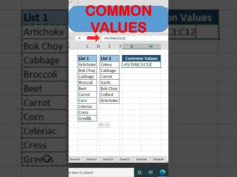
Find Common Values From Two List In Excel @BrainUpp
 0:01:55
How to Use Excel to Match Up Two Different Columns : Using Excel & Spreadsheets
 0:03:34
Compare Two Columns in Google Sheets and Highlight Differences Using Conditional Formatting
 0:00:32
#ExcelShort19 - Excel Trick To Compare Two Different Columns To Identify Differences
 0:03:50
How to compare two columns in different Excel sheets using Vlookup
 0:08:25
How to Compare Two Columns In Excel? | Compare Excel Columns for Matches & Differences | Simplil...
Комментарии