filmov
tv
How to Perform a Convolution in MATLAB | MATLAB Tutorial

Показать описание
Convolutions in MATLAB! How to take the convolution conv() of two functions f(t)*x(t) to generate a system response. Discrete functions and smoothing curves discussed with examples.
OVERVIEW
conv(a,b) is used to take the convolution of two functions. Be sure to scale your output! 3:06
If you want the output to have the same number of terms as 'a', use conv(a,b,'same').
CHAPTERS
0:00 Introduction
0:36 Part 1: Convolution of Two Functions f(t)*g(t)
1:57 Using conv()
2:25 Analyzing System Response
3:06 Scaling System Response
7:24 Part 2: Smoothing Curves
9:13 Using conv(a,b,'same')
MATH CORRECTIONS/COMMENTS on the video -- PLEASE READ!!
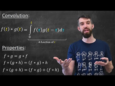
1. f(t)*g(t) is said "f convolved with g".
2. at 4:15 we see the max value of the output = max f(t) times max g(t) -- know that this does not always happen.
3. Scaling the t-axis / x-axis is not always straightforward. My scale and shift works in this case but doesn't apply to the general case.
4. at 5:50 you don't need the .* for (1:length(yt))*dt because this is a vector times a scalar.
5. at 6:50 take note I have only included the t2(1) term. However, for the general case, you may use t2(1) + t1(1) to account for your signals starting at different times. In this video, t1(1) was simply zero and thus adding only t2(1) worked.
MORE MATLAB
LIKE AND SUBSCRIBE
If you received something of value from this video, please like and subscribe to support this channel :) as always comment below and I will answer your question!
OVERVIEW
conv(a,b) is used to take the convolution of two functions. Be sure to scale your output! 3:06
If you want the output to have the same number of terms as 'a', use conv(a,b,'same').
CHAPTERS
0:00 Introduction
0:36 Part 1: Convolution of Two Functions f(t)*g(t)
1:57 Using conv()
2:25 Analyzing System Response
3:06 Scaling System Response
7:24 Part 2: Smoothing Curves
9:13 Using conv(a,b,'same')
MATH CORRECTIONS/COMMENTS on the video -- PLEASE READ!!
1. f(t)*g(t) is said "f convolved with g".
2. at 4:15 we see the max value of the output = max f(t) times max g(t) -- know that this does not always happen.
3. Scaling the t-axis / x-axis is not always straightforward. My scale and shift works in this case but doesn't apply to the general case.
4. at 5:50 you don't need the .* for (1:length(yt))*dt because this is a vector times a scalar.
5. at 6:50 take note I have only included the t2(1) term. However, for the general case, you may use t2(1) + t1(1) to account for your signals starting at different times. In this video, t1(1) was simply zero and thus adding only t2(1) worked.
MORE MATLAB
LIKE AND SUBSCRIBE
If you received something of value from this video, please like and subscribe to support this channel :) as always comment below and I will answer your question!
 0:23:01
But what is a convolution?
 0:14:02
Convolution in 5 Easy Steps
 0:05:06
2D Convolution Explained: Fundamental Operation in Computer Vision
 0:05:36
What is convolution? This is the easiest way to understand
 0:10:33
The Convolution of Two Functions | Definition & Properties
 0:15:56
Convolution integral example - graphical method
 0:00:55
What is Convolution
 0:00:21
Convolution Tricks || Discrete time System || @Sky Struggle Education ||#short
 6:38:44
Train a Convolutional Neural Network from Scratch PyTorch, Next js, React, Tailwind, Python 2025
 0:06:47
Convolution Part 1: What is Convolution
 0:30:42
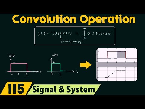
Introduction to Convolution Operation
 0:10:58
Tutorial 21- What is Convolution operation in CNN?
 0:06:21
What are Convolutional Neural Networks (CNNs)?
 0:09:59
What is Convolution and Why it Matters
 0:10:10
Discrete Time Convolution Example
 0:11:05
How to Perform a Convolution in MATLAB | MATLAB Tutorial
 0:10:47
Convolutional Neural Networks Explained (CNN Visualized)
 0:20:05
How Convolution Works
 0:07:55
Convolution and the Fourier Transform explained visually
 0:10:58
Convolution Operation in CNN
 0:15:48
What is Convolution? And Two Examples where it arises
 0:04:34
Convolution Explained - Signal Processing #24
 0:07:17
The convolution operation in machine learning
 0:07:49
Method to Find Discrete Convolution
Комментарии