Excel SUMIF Function Explained - Financial Modeling Tutorial

Excel SUMIF Function Explained is a free tutorial by 365 Careers from Financial Modeling course
Link to this course(Special Discount):
This is the best Financial Modeling Course
Course summary:
Master Microsoft Excel and many of its advanced features
Become one of the top Excel users in your team
Carry out regular tasks faster than ever before
Build P&L statements from a raw data extraction
Build Cash Flow statements
Discover how to value a company
Build Valuation models from scratch
Create models with multiple scenarios
Design professional and good-looking advanced charts
English
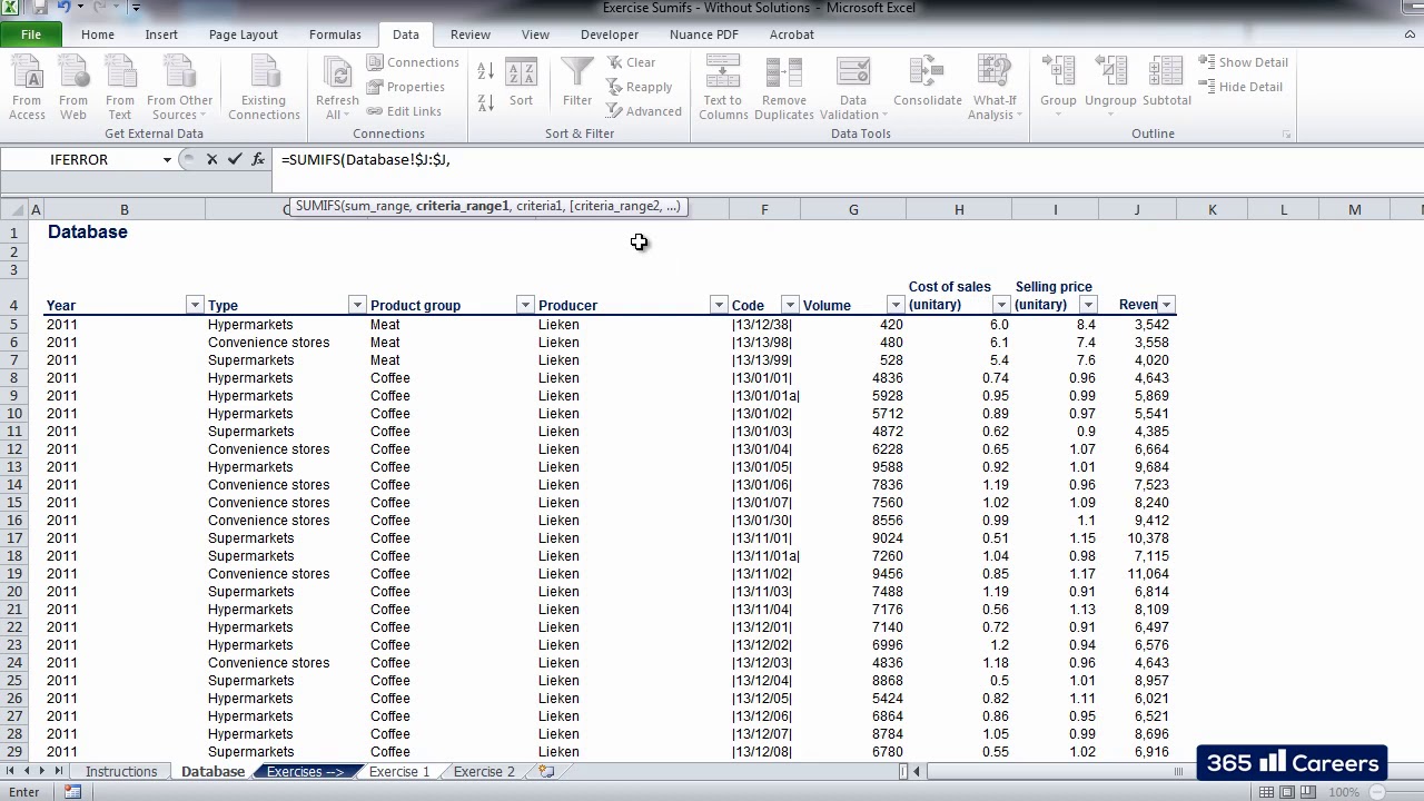
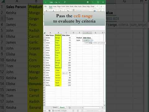
Hello and thank you for joining! This is our update from the 16th of December. We recommend that you try to visit the course at least once every week or two, because it is likely that you'll find new lessons, exercises or materials. Having said that, let's start with the core part of this lesson - solving the exercise that was uploaded in Course Materials. This exercise is dedicated to the application of the ""Sumifs"" function. In the first part of the course we saw how ""Sumifs"" works and now it is time to see how it is applied in practice. Let's open the exercise file. In its first sheet we find the instructions, which are quite simple. The ""Database"" sheet contains data for transactions carried out in a chain of supermarkets. We have to use this information in order to fill in the two tables that are in the ""Exercise 1"" and ""Exercise 2"" sheets with an annual breakdown of revenues. The information in ""Database"" is organized in a table format and consists of more than 15,000 rows. This does not scare us, right? We know how to deal with large quantities of data. Let's insert a filter, as it is much easier to work once we've done that. I'll use the Alt + A + T shortcut in order to carry out the command faster. It is always a good idea to spend an extra minute looking through the material in order to get a better understanding of the data source. Let's go through the source table and describe the type of information that it contains. The first column shows the financial period in which the transactions in each row occurred. The ""Database"" contains transactions from four periods' 2011, 2012, 2013 and 2014. In column C we can see the type of the store in which the transactions were carried out. There are three types of stores: ""convenience stores, ""hypermarkets"" and ""supermarkets"". The next column contains a product group classification: ""meat, ""coffee"" ""alcohol, etc. Column E provides information about the producer of the products, while column F contains an internal code used by the accounting department of the firm in order to classify all items. We're not going to use it in this exercise. In the last four columns we have data about the number of units that were sold, the unitary cost of the items, the unitary price at which they were sold and the amount of revenue that was registered given by the product of volume and unitary selling price. The only figures that we will need for this exercise are the ones in the last column - revenues. Now that we've done our initial screening, we can go ahead and solve the exercises in exercise one we have to fill in a table with the amount of revenues that each of these product groups had throughout the four financial periods. ""Sumif"" would not be sufficient for this task. We need to work with multiple conditions, hence ""Sumifs"" comes into play. Above each of the financial periods let's type the format that was used in our ""Database"". By doing this we will be able to use the cells as criteria in the ""Sumifs"" function. We have 2011, 2012, 2013 and six months of 2014. The first argument of ""Sumifs"" is the sum range. That will be column J in the source sheet - Revenues. Let's select the whole column J and fix it. Then we have to pick the range of our first criteria. Given that we have to find revenues of each product group, I suggest that we select the column containing product groups - column D, I am fixing column D as well. Back to our output table. The ""product group"" criterion lies in B5. Let's fix its column reference. Good. This was our first criterion. Now we have to include a second one. The range for our second condition is column B in the ""Database"" sheet, where we have the year in which a given transaction occurred. Then we can go back to the ""Exercise 1"" sheet and select C3 as a criterion, which is the respective financial period. Let's fix the row reference of the cell. I am doing this, because later when we copy the function downwards, we want our criterion to remain in the third row. We will not fix the column reference, because we want the criterion to