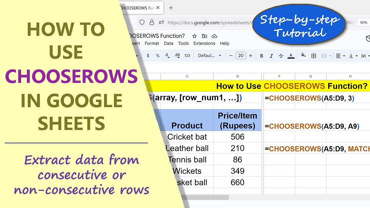
Google Sheets | CHOOSEROWS | Function | Extract Data | Example | Spreadsheet | Step-by-Step tutorial

What does the Google Sheets CHOOSEROWS function do? It creates a new
array with the data extracted from the rows of the specified range.

The two mandatory arguments CHOOSEROWS require are: array and row_num1.

=====================================
Food & Health Series Using 2D Animation

All the Parts of How to Prevent Diabetes series is based on research findings.

How to Prevent Diabetes Part 1

How to Prevent Diabetes Part 2

How to Prevent Diabetes Part 3

How to Prevent Diabetes Part 4

How to Prevent Diabetes Part 5
=====================================
-------------------------------------
How to Use FACT and FACTDOUBLE in Google Sheets?

Use FACT and FACTDOUBLE to get the factorial and double factorial of a number:

-------------------------------------
How to Use PERMUT and COMBIN in Google Sheets?

Get the permutations and combinations of n objects:

-------------------------------------
How to Use SUMSQ in Google Sheets?

Use SUMSQ function to calculate the sum of squares of n numbers:

-------------------------------------
How to Use SUMIFS in Google Sheets?

Use SUMIFS to add numbers based on two or more conditions:

-------------------------------------
How to Use XLOOKUP for Reverse Search in Google Sheets?

XLOOKUP can search for the search key in the regular or reverse order in the lookup range:

-------------------------------------
How to Use LAMBDA and BYCOL in Google Sheets?

Create and test your own function using LAMBDA, and then use your function in a function like BYCOL:

-------------------------------------
How to Use XMATCH in Google Sheets?

XMATCH returns the position of the specified search key in a row or column:

-------------------------------------

CHOOSEROWS Function Formula

=CHOOSEROWS(array, [row_num1, …])

Start the formula with an equal-to symbol.

CHOOSEROWS is the name of the function.

array is the range with one or more rows.

row_num1 is the row number of the array from which to extract data.

row_num1, can be, for example, a hard-coded number, cell address, or function that returns a number.

row_num2, row_num3, and others are optional and are row number 2, 3, and others.

Examples

Example 1

=CHOOSEROWS(A3:A7, 3)

The above function formula will return the data in row number 3 of the array A3 to A7.

Example 2

=CHOOSEROWS(D12:H25, C12, C14, C15)

Assume that cells C12, C14, and C15 have values of 5,7, and 8 respectively. CHOOSEROWS will return the data in rows 5, 7, and 8.

Example 3

=CHOOSEROWS(A3:A15, MATCH("inventory", A3:A15), 7)

For the row_num1 argument of CHOOSEROWS, the MATCH function is substituted and this function returns the position of the search key inventory, if found, in the range A3 to A15. Say MATCH returns 3. Then, CHOOSEROWS will return data in row 3 and row 7 of the range A3 to A15.

Take a look at this video tutorial, which gives the steps to use the Google Sheets CHOOSEROWS function with examples.