Google Sheets | HSTACK | Function | Formula | Example | Spreadsheet | Tutorial | Append Range

The Google Sheets HSTACK function returns an array, appending one or
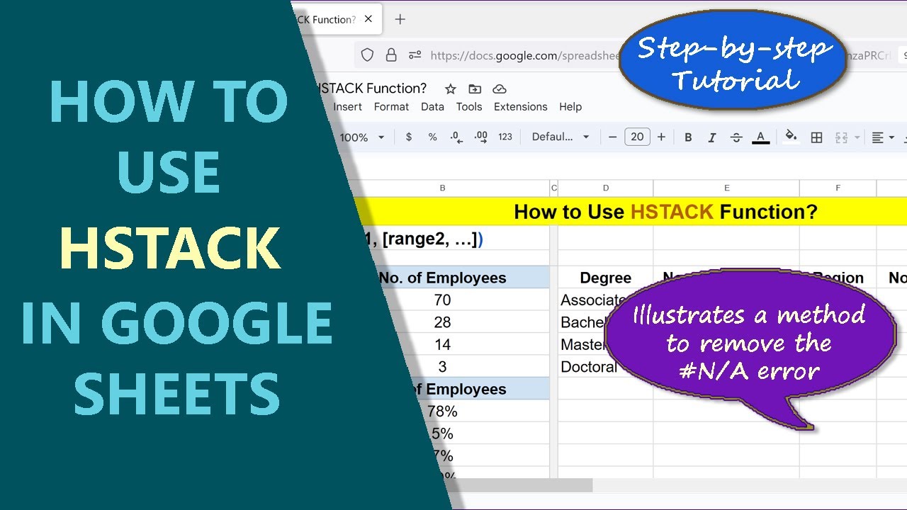
more ranges to the first range horizontally and sequentially. If you wish to combine two or more ranges of data into one range, with the data stacked horizontally, you may want to consider the HSTACK function. Take a look at this spreadsheet tutorial, which gives the steps to use HSTACK with examples.

=====================================
Food & Health Series Using 2D Animation

All the Parts of How to Prevent Diabetes series is based on research findings.

How to Prevent Diabetes Part 1

How to Prevent Diabetes Part 2

How to Prevent Diabetes Part 3

How to Prevent Diabetes Part 4

How to Prevent Diabetes Part 5
=====================================

-------------------------------------
How to Use VSTACK in Google Sheets?

Use VSTACK to append data to a range vertically:

-------------------------------------
How to Use WRAPCOLS in Google Sheets?

Wrap data in a row into one or more columns:

-------------------------------------
How to Use WRAPROWS in Google Sheets?

Wrap data in a column into one or more rows:

-------------------------------------
How to Use CHOOSECOLS in Google Sheets?

Get the data from one or more columns, using CHOOSECOLS:

-------------------------------------
How to Use CHOOSEROWS in Google Sheets?

Extract one or more rows of data using CHOOSEROWS:

-------------------------------------
How to Extract Specific Data Using CHOOSEROWS and MATCH in Google Sheets?

Extract data pertaining to specific strings, using CHOOSEROWS and MATCH functions:

-------------------------------------
How to Use TO_PERCENT in Google Sheets?

Format numbers with percent symbol using the TO_PERCENT function:

-------------------------------------
How to Use XMATCH in Google Sheets?

XMATCH returns the position of the specified search key in a row or column:

-------------------------------------

If the ranges you want to append are of different sizes, then the HSTACK function will fill the extra cells with the #N/A error.

HSTACK Function Formula

=HSTACK(range1, [range2, …])

Start the formula with an equal-to symbol.

HSTACK is the name of the function.

range1 is the first range to which range2 will append horizontally.

range2 and others are optional, and are the second and other ranges
that will append to range 1 horizontally and sequentially.

Examples

Example 1

=HSTACK(A2:B5, A7:B10)

The function will return an array, which will be the combination of the two ranges A2 to B6 and A7 to B11. This range will append to the first range horizontally.

Example 2

=HSTACK(A2:B6,A7:B10)

The first range has one row more than the second and because of the
difference in the range sizes, HSTACK function will fill the extra cells
with the #N/A error.

Checkout this video tutorial, which gives the steps to use the Google Sheets HSTACK function with examples.