Linear Differential Equations & the Method of Integrating Factors

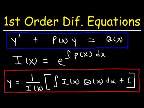
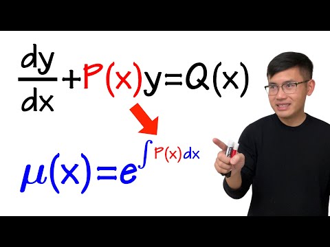
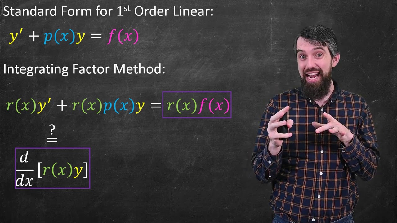
Linear first order differential equations are particularly nice because we have a method called integrating factors that lets us solve every single first order linear ODE. We will define what makes a differential equation linear, derive the formulas for the integrating factor and the solution, and then talk about the existence and uniqueness theorem that is implied by this.

0:00 Linear ODEs
4:06 Integrating Factors
10:50 Existence & Uniqueness

OTHER COURSE PLAYLISTS:

OTHER PLAYLISTS:
► Learning Math Series
►Cool Math Series:

BECOME A MEMBER:

MATH BOOKS & MERCH I LOVE:

SOCIALS:

[aakashSky-]

Sir may you and your family live happily forever. such quality material you are providing us for free....Damnn this is so much better than the paid courses...Thanks a lot sir.

[julianyerger]

As an Electrical Engineering sophomore struggling through differential equations, thank you for making these videos! They were also very helpful for my Calc 3 class last year. This is by far my favorite math channel on YouTube, your explanations are great!

[clashfun]

u maths teacher from other countries are literally awesome and stand much above our indian teachers in explaining.

Thanx for such a beautiful explaination

[zandiviljoen]

Sir I just want to thank you so much for doing these videos. I am studying engineering and because of covid we started a lot later this year and as a result rushed through a lot of the beginning stuff. Because of this I was struggling to keep up and struggling to build on my very 'un-established' foundations of differentials. Your vids allow me to understand concepts better and rewind when I don't and I really really appreciate it. Love and appreciation from South Africa!!

[drkknght]

Sometimes I wonder why we can't get this type of professor in our college and school?

[marvelousjames]

This is absolutely fantabulous. Currently revising ODEs for PDEs and this series has done wonders. Especially this video on Integrating factors, very sound explanations all through. You've done a wonderful job and I hope you're aware that is highly appreciated.

[hrkalita]

Please make a video on tensors used in general relativity 🙏🙏💓

[intelligentdonkey]

Sir you and Grant Sanderson(3b1b) Sir are the persons who made me love the subject which I hated the most.❤️thank you so much....Love from India

[angelmendez-rivera]

I would like to add that there is another formulation of this idea which, while I admit it is potentially less intuitive, it is more easily generalizable to higher-order equations, and it shows the true connection that this subject has with linear algebra, which in turn, may make it more illuminating.

Linear first-order equations can be written as D[y(x)] + p(x)·y(x) = q(x), as explained in the video, where D[y(x)] stands for the derivative of y. It will make sense why I am using this notation instead of the usual y' in just a moment, but bear with me. Notationally, you may be tempted to "factor out" the y from the right, writing this as [D + p(x)][y(x)] = q(x), and if you rename the object A := D + p(x), then you get an equation that looks like A[y(x)] = q(x). Now this looks a lot more like an equation you would encounter in linear algebra: y and q are functions, and A is some type of object that behaves like a linear operator acting on the space of differentiable functions, so in a meaningful sense, A is very much analogous to a matrix here. This representation makes it obvious what is it that you need to do to solve the equation: you want to "invert" the linear operator A, find some A^(–1), so that y(x) = [A^(–1)][q(x)] is the solution to the equation. For p(x) = 0 for almost all x, this is implies A := D, and so finding A^(–1) is trivial: you simply integrate using the initial conditions. However, for any other p(x), this is completely non-obvious.

This is where the integration factors comes into play. It is not obvious how to invert an operator that looks like D + p(x), but if you could somehow reexpress A[y(x)] as [r(x)^(–1)·D][r(x)·y(x)], then this would make the problem trivial again. What this video does is precisely teach you that you can always do this: if r(x) = exp(Antiderivative[p(x)]), then you can always write D[r(x)·y(x)] = r(x)·q(x), which is indeed equivalent to r(x)^(–1)·D[r(x)·y(x)] = q(x). Why do I want to rewrite A[y(x)] as r(x)^(–1)·D[r(x)·y(x)]? Before I explain this, let me make one final change to the notation. Let the linear operator R be defined by the rule R[y(x)] = r(x)·y(x). Hence r(x)^(–1)·D[r(x)·y(x)] = [R^(–1)·D·R][y(x)] = q(x). Now it should become clear why I wanted to rewrite A[y(x)] as [R^(–1)·D·R][y(x)]: because this is just the same as saying that A = R^(–1)·D·R, where A, D, R are linear operators. Notice how this is exactly analogous to the diagonalization of a matrix into a diagonal eigenvalue matrix and an eigenvectit matrix. In effect, using integration factors in the study of differential is just a "diagonalization" of the operator A := D + p(x), which is the operator we want to invert. With this, solving the equation is now trivial, and the solution becomes y(x) = [R^(–1)·D^(–1)·R][q(x)] = 1/r(x)·Integral[r(x)·q(x)], which is exactly what we obtained in the video! Of course, I am being somewhat handwavy here, since technically, D is not an invertible operator in the ordinary sense, and so D^(–1) here represents integration with usage of a specific initial condition, but the core idea is still the same: solving a linear differential equation is just diagonalizing the operator A. It is, indeed, just linear algebra, and this is the hidden truth that I have been trying to uncover here in my explanation.

This formulation is not only illuminating as to the linear-algebraic nature of these equations, but it is easy also useful, because it gives us a method by which you can solve linear equation of higher-order in terms of this first-order idea, as long as you are able to "factorize" the equation. What do I mean by this? As an example, suppose you have an equation y''(x) + f(x)·y'(x) + g(x)·y(x) = h(x), which, for reasons that now should have become apparent, I should rewrite as [D^2 + f(x)·D + g(x)][y(x)] = h(x). Again, with A := D^2 + f(x)·D + g(x), this is just A[y(x)] = h(x), a linear equation, and you want to "invert" A so that the solutions look like y(x) = [A^(–1)][h(x)]. Here, A is again a linear operator, but this time, it is equal to a quadratic polynomial in D instead of a first-degree polynomial in D. Here is the inspiration: if polynomials with complex coefficients can be always factored into a product of polynomials of first-degree with complex coefficients again, then, should we not be able to do the same thing with polynomials in D with functional coefficients? The answer is yes, with a large caveat: this "multiplication" of linear operators, which are comprised of sums of products of D and functions, is not commutative. This is to say, R·D is not the same as D·R: again, entirely analogous to matrix multiplication in linear algebra. Thus, the order in which you do the factorization matters, and this can also complicate things. To see this explicitly, you can carefully evaluate {[D – r(x)]·[D – s(x)]}[y(x)] as [D – r(x)]{D[y(x)] – s(x)·y(x)} = D{D[y(x)] – s(x)·y(x)} – r(x)·D[y(x)] + r(x)·s(x)·y(x) = (D^2)[y(x)] – D[s(x)·y(x)] – r(x)·D[y(x)] + r(x)·s(x)·y(x) = (D^2)[y(x)] – D[s(x)]·y(x) – s(x)·D[y(x)] – r(x)·D[y(x)] + r(x)·s(x)·y(x) = {D^2 – [r(x) + s(x)]·D + [r(x)·s(x) – s'(x)]}[y(x)]. This gives you the factorization D^2 – [r(x) + s(x)]·D + [r(x)·s(x) – s'(x)] = [D – r(x)]·[D – s(x)], and the lack of commutativity is manifested in the asymmetric expression r(x)·s(x) – s'(x). Anyhow, the idea is that, in factorizing the quadratic polynomial A as [D – r(x)]·[D – s(x)], you can write A as R1^(–1)·D·R1·R2^(–1)·D·R2, where R2 is the operator that multiplies its input by the function exp(–Antiderivative[s(x)]), and R1 is the operator that multiplies its input by the function exp(–Antiderivative[r(x)]). The same idea applies for higher-order equations, where you factorize higher-degree polynomials in D. What does this mean? It means that solving any linear equation, in theory, merely reduces to multiplying by an appropriate integration factor, integrating, and repeating the process, and this can be done in the other direction too, by simply substituting y(x) with the appropriate t(x)·y(x) for some factor t, and proceeding from there. You may not even need to factor the equation, you only need to know that you can always find the appropriate integration factor, because this idea guarantees its existence.

This idea is what makes linear equations so much simpler to solve than non-linear ones in general. This idea also opens the door to the discipline of mathematical study known as operator theory, where a treatment of rigor is given to these ideas of linear operators, expanding these concepts beyond the linear algebra of matrices and Euclidean R^n spaces. This turns out to have significant applications in the sciences, especially in quantum physics, but it also useful fir the study of other disciplines in mathematics, in turn.

[mr.dynamite]

Always great when you can find a video like this if your calculus textbook doesn't explain it clearly. Abstract concepts like this are hard for me to grasp but watching this only 3 times was enough for me to understand it perfectly. 10/10

[naiko]

Note that the integrals along the way generate a few constants, but they all end up absorbed in the final constant anyway, that's why they weren't mentioned.
The sign when we get rid of the absolute value in e ^ ln |r(x)| is ultimately also absorbed into the constants of integration.

[watsoncrick]

Wow...thank you so much...I think nobody else could be this much clearer

[jamesmarshel]

It seems like you used "wishful thinking " when you said "I would love ..." It's one of my favorite problem solving strategies. I wish my teachers would have made this technique (and others) more explicit when I was in highschool/college. It makes motivating proofs easier for everyone. Loved the lecture. Got hooked by your calculus series.

[monadic_monastic]

Hi Dr. Trefor, I'm told from the grapevine that the (first-order linear) ODEs which are amenable to the method of integrating factors are in fact 'non-exact' diff eqs that can be turned into exact diff eqs precisely from this integrating factor.

If there's no misconception there or if I'm missing anything out, then this picture also leans heavily on the math of differential 1-forms, which have an isomorphism with vector fields, and it turns out exact diff. forms have a correspondence with conservative vector fields. (and I'd assume vice versa: non-exact diff forms correspond to non-conservative vector fields)

In that case then with that geometric picture/correspondence in mind, since we have that exact diff eqs/exact diff forms <=> conservative vector field picture in mind, then by turning a non-exact diff eq./form into an exact one via these integrating factors, aren't we dually in the process also turning a non-conservative vector field into a conservative one?

I'd like to know more about this potential (no pun intended) geometric correspondence.

[cinderellachirwa]

This was posted a year ago 😂and I can't help but thank God cause it's helped me so much 😂all our teacher said was to memorize and it really didn't make sense but you 😂😂you came like a hero 🔥💯

[Junker_]

You are a stellar teacher. Thank you for all the help you have given me.

[lumbradaconsulting]

How cool. The key part for the development of the method is the dot product of the derivative ! Thank you

[EggZu_]

i've had integrating factors explained to me 3 times now and it always impresses me haha
great video thank you

[johnlee-dvcd]

You always know what we confuse about. You are a great and amazing teacher.

[georgesadler]

Professor Bazett, thank you for an excellent analysis and derivation of Linear Differential Equations and the classical Method of Integrating Factors.