How to Compare Two List and Highlight Unique Values

#Excel #ExcelTipsandtricks #highlightuniquevalues

You have a table and you don't find duplicates, rather than you want to find unique values from both the data by comparing it.

You can do this by using countif and conditional formatting.

construct the table first. Name the table using name box. This will help you to just select it every time rather than entering the details.

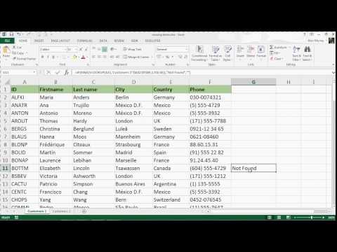
Input the countif formula next to the table. Enter the below formula.
=countif(list_1,d3)

List_1 is the name range. D3 is the cell reference of the second table. This may change based on your second table details.

Once the formula is supplied, it would return us either 1 or 0. When it finds the same result, it would return 1 .

when the result is not found (Unique Value), it would return us 0.

Method 2 :

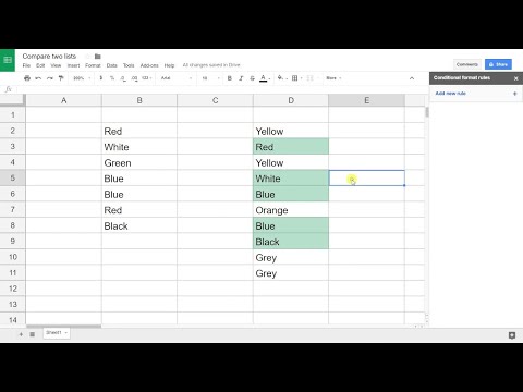
Select the data .Go to Home, navigate through conditional formatting, pick new rule and choose formula to determine which cell to format.

Enter the countif formula

=countif(list_1,d3)=0.

The above formula is used to determine true or false value. when the value is true,highlight the cell.

It is up to to the user to determine to choose which formula to use.

Keep Watching,Keep learning.

[akashthakur]

Awesome video mam it is so useful for me please keep it up in future thanks for making video

[aravindify]

Extraordinary tutor... but one only small backlog is show the full screen of excel then it will be beneficial for the viewers without any doubts in the tabs👏🏻keep on