filmov
tv
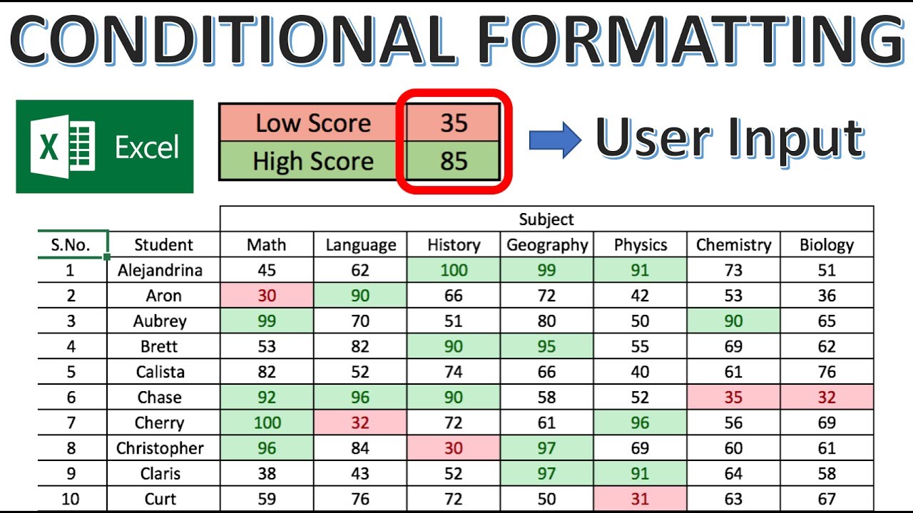
Excel Conditional Formatting Based on Another Cell Tutorial
Показать описание
Quick Tutorial of Excel Conditional Formatting based on another Cell Value (can be changed by the user)
Recommended Gadgets/Products:
Products:
Check the below Playlists..
Excel Tutorials:
Excel Chart Tutorials:
Excel Pivot Table Tutorials:
Excel Gsuite Tutorials:
Excel Tips & Tricks:
Powerpoint Tutorials:
Gadget Reviews:
Thanks for watching!!! 😊🙏
Please do Subscribe and Hit the Bell 🔔icon to support my efforts and to receive all my videos Notifications.
Follow me on below to stay connected👇
 0:09:40
Excel Conditional Formatting with Formula | Highlight Rows based on a cell value
 0:09:29
Excel How To: Format Cells Based on Another Cell Value with Conditional Formatting
 0:06:43
Conditional Formatting in Excel Tutorial
 0:10:37
Master Conditional Formatting in Excel (The CORRECT Way)
 0:04:25
Conditional Formatting Formulas - Mystery Solved with 3 Simple Rules
 0:01:30
Excel Conditional Formatting based on Another Cell | Highlight Cells
 0:00:29
Conditional Formatting in Excel | Highlight Marks Pass/Fail #shorts #excel
 0:05:20
MS Excel - Advanced Conditional Formatting
 0:02:01
How to Use Conditional Formatting with Drop-Down Lists in Excel (FREE TEMPLATE RO TRY)
 0:03:46
Excel: Conditional Formatting
 0:06:54
Excel Essentials -- Level UP! -- Conditional Formatting for Due Dates and Expiration Dates
 0:04:16
Excel Conditional Formatting Based on Another Cell Tutorial
 0:17:39
Excel Conditional Formatting in Depth
 0:12:00
5 Conditional Formatting tips to make you a rock star at work 🤘
 0:05:51
Excel Conditional Formatting Advanced Technique
 0:04:21
Apply Conditional Formatting to an Entire Row - Excel Tutorial
 0:20:59
Conditional Formatting in Excel | Excel Tutorials for Beginners
 0:06:30
Excel - Advanced Conditional Formatting with sample Excel file - 3 examples
 0:03:42
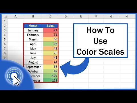
How to Use Color Scales in Excel (Conditional Formatting)
 0:10:42
MS Excel - Conditional Formatting Part 1
 0:04:36
Conditional Formatting Based on Specific Text in Microsoft Excel! Format Good as Green. #howto #wow
 0:25:18
Excel Conditional Formatting (Overview + Advanced Examples)
 0:09:23
Excel Conditional Formatting using Formulas
 0:05:02
Advanced Conditional Formatting in Excel | Conditional Formatting in Excel
Комментарии