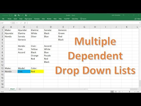
How To Create MULTIPLE Dependent Drop-Down Lists in Google Sheets

Looking to create advanced drop-down lists in Google Sheets? Dive into this tutorial to learn how to set up multiple dependent drop-down lists efficiently, perfect for intricate data entry tasks.

✨ Key Highlights:
▪️ Setting Up the Master Data: Understand how to organize your master data, which forms the basis of your dependent drop-down lists.
▪️ Creating the First Drop-Down List: Learn the steps to create your primary drop-down list, which will determine the content of subsequent dependent lists.
▪️ Using Data Validation for Dependent Lists: Discover how to use Google Sheets' data validation feature to create dependent lists that change based on the selection in the first list.
▪️ Data Preparation for Multiple Lists: Explore how to use the INDEX and MATCH functions to prepare data for multiple dependent lists.
▪️ Transposing Data for Horizontal Display: Find out how to use the TRANSPOSE function to display your drop-down lists horizontally for a cleaner look.
▪️ Dealing with Dynamic Ranges: Get tips on adjusting your data validation ranges for each row to ensure each drop-down list functions correctly.

00:00 How To Create Multiple Dependent Drop Down Lists in Google Sheets
01:25 Create First Drop-Down List in Google Sheets
02:58 Create Dependent Drop-Down List in Google Sheets
04:46 Create Multiple Dependent Drop-Downs in Google Sheets

🚩Let’s connect on social:

Note: This description contains affiliate links, which means at no additional cost to you, we will receive a small commission if you make a purchase using the links. This helps support the channel and allows us to continue to make videos like this. Thank you for your support!

#googlesheets

[LeilaGharani]

GOOD NEWS! The invisible dollar sign issue is fixed! We can see the $ signs in data validation and we can remove them. So you can skip the part where I update each cell reference and just remove the dollar signs from the first dependent validation, and then copy the data validation down (Works like Excel now 😉)

[ranjansingh]

Hi Leila,

You can remove the $ sign from validation and copy-paste, it will change the range as expected, which can be used for huge data set.

[mreighties]

Hi Leila,

Google now lets you create a drop-down using "Relative cell referencing" like you created using the range "Master!F4:Z4 and now you can drag the drop-down down and the range will change for each row without having to "update" each data validation.

When you create the drop-downs for the "Categories" in column A then make sure the first one uses "Absolute cell referencing" so that when you copy or drag the drop-down down into the cells below the "cell referencing" will be locked and not change.

But when you create the "dependent drop-downs" in column B then create the first drop-down and then look back at it and make sure the "cell referencing" is set to "relative" by removing the $ signs. Then copy or drag down that drop-down to the cells below. The drop-downs will change without having to update each one.

James :)

[biljanapesevska]

It took me a total of 3 hours to actually create a dependant dropdown, and only 10 minutes after stumbling upon your video! Thanks! I wish I found your video first!

[vidulaworlikar]

Hi, I have a suggestion. After copy-pasting the formula for data validation, instead of manually changing the cell row number in the last step - you may just open the data validation formula from any one of the pasted formulas (say 5th row). Remove the $ sign next to the cell number (keep column frozen) - for example: Sheet1!$K5:$N5 (originally it was Sheet1!$K$5:$N$5). Now you will get a popup asking if you want to make the same change to all the cells - and viola - it changes to respective row numbers. No need to manually change each and every formula.

[maeobuyes]

From all the videos I've browsed yours was the most honest especially on the limitations. Other videos dont talk about it and how to deal with it. Your video was easy to follow and provided the solution to my problem. Thank you.

[averie]

I found an easier way to update all the formulas, instead of manually typing each number into the data validation. Basically, if you save the data validation and then go back, the $'s pop up and you can delete them. This worked for me, not sure if it will work for others. Instructions below. (Edit: Clearer instructions)

At 5:42, she talks about invisible dollar signs stopping us from copying the data validation formula all the way down on the "Dep. List" sheet for row B. I followed her instructions from 6:00 to 6:15, and then I copied ONE cell only (unlike how she does all of them at 6:35) and pasted it into cell B4. I reopened the Data Validation for B4 and I could see all the $ signs. I manually deleted each one, and saved.

NOTE: Make sure that you click on the text itself when erasing the $s-- do not click on the little box that looks like four squares that says "Select Data Range." If you click on that, it makes a new pop-up window, and it puts the $s back every time. Very frustrating if you keep deleting them.

Then I copied the B4 formula all the way down, and it automatically changed all the numbers. I checked each cell; they all worked right. It was much faster than what she did from 6:44 to 6:51. I'm guessing that the "invisible dollar signs" are actually just auto-filled behind your back -- you see them if you reopen the formulas.

Hope this helped someone!

[bobbyman]

You honestly deserve more than 1 million subscribers.. Let's all make that happen

[tynerds]

A huge thank you for these guides! They are really easy to follow!

[westernugmedia.]

Leila, I like the way u speak out your English .. It's, favourable for us all. Even here in Africa

[lovelyraincoat]

This is brilliant, I'm just starting to learn and there's no way I could have put all those formulas together. Thank you so much!!

[TylerStanczak]

This is awesome! Thanks for sharing this tutorial on drop-down lists :)

[MsEteria]

This is lifesaver!! I watched 10 other videos and I was going crazy. And you made it super easy. Thank you, thank you, thank you

[JohnDeir]

Actually you can put formulas in Google sheets validations. And the best trick is to make name range of cells listed below each category name. So under Productivity you create a name range called "Productivity" and so on. Then you can create a formula in data validation associating the category with the name range. Lots easier and try it out. Great tutotial, just trying to help.

[joshedgerly]

You are an absolute life saver — I cannot thank you enough for this!

[jenniferblanchard]

Is there a way to pull the information on "notes" or "comments" linked to the extracted column? I really liked your video. Thank you so much.

[joanmayes]

Love your videos. You explain things very clearly with good examples. Can a 3rd column be created and linked to the 2nd dynamic dropdown, creating a 3rd choice based on the second choice?

[taniknight]

Awesome tutorials! I was SO glad to discover that dragging these vlaidations down now works. I have a big data set to work on (auto categorisation of bank transactions) and this has made a drop down list style of data entry possible.

[luks]

If you go into the second data validation, you can actually remove the $ and simply copy and paste the validation. Thanks for the tutorial!

[Chander-gyxz]

@Leila the invisible $ problem in Google sheet can be solved by putting the $ sign for the Data Validation you have done for the first row and then remove the $ and save the Data Validation.

Now if you drag down the Data Validation it will automatically extend the selection. I have tried it out and it works