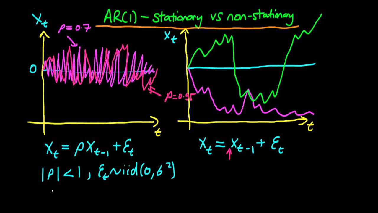
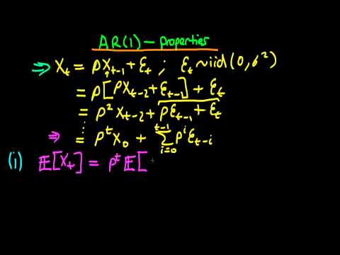
The qualitative difference between stationary and non-stationary AR(1)

This video explains the qualitative difference between stationary and non-stationary AR(1) processes, and provides a simulation at the end in Matlab/Octave to demonstrate the difference.

clear; close all; clc;

n=10000; % Setting the number of time periods equal to 10000.
b=1;
rho=1; %This is the coefficient on the lagged part of x

x=zeros(n,1); % Initialise the vector x
x(1)=0;

for i = 2:n
x(i)=rho*x(i-1)+b*randn();
end

zoom=1.0;
FigHandle = figure('Position', [750, 300, 1049*zoom, 895*zoom]);
plot(x, 'LineWidth', 1.4)
ylabel('X(t)')
xlabel('t')

I also include the same in R (Courtesy of Jesse Maurais):

z = rnorm(1000)
gen = function(rho) {
x = numeric(length(z))
x[1] = z[1]
for (i in 2:length(z)) {
x[i] = rho*x[i-1] + z[i]
}
x
}
display = function(rho) {
x = gen(rho)
lines(x)
}
for (it in 1:100) {
display(it/100)

[SpartacanUsuals]

Hi, glad to hear you liked it. I will add that suggestion to my list! Thanks, Ben

[JesseMaurais]

I just mocked up a similar simulation in R, but I animated it, increasing rho by 0.01 from 0 to 1 in each frame, at 2 frames per second, using the same white noise data. Watching how the data changes makes a lot more sense now. Thanks for the videos. 

[debashisbanerjee]

Amazingly explained. Probably the best video on this topic on internet.

[tonyfang]

Sketched the same thing in Python, hope it helps!

import numpy as np
import pandas as pd
import matplotlib
import matplotlib.pyplot as plt

# define each datapoint as a normal r.v.
def generate_datapoint(params):
mu = params[0]
sigma = params[1]
return np.random.normal(mu, sigma)

# Set the number of datapoints
T = 100

B = pd.Series(index=range(T))
B.name = 'B'

for t in range(T):
# Now the parameters are dependent on time
# Specifically, the mean of the series changes over time
params = (t * 0.1, 1)
B[t] = generate_datapoint(params)

plt.plot(B)
plt.xlabel('Time')
plt.ylabel('Value')
plt.legend(['Series B']);

[asadkhanbb]

@Ben Lambert, I got addicted to your videos on Econometrics. Thanks

[MrScattterbrain]

Ben, thank you so much for these videos on time series. And, in particular, for this one. This answered all little confusions and doubts that I used to have.

[harshitnarula]

Wow this is really helpful..ive been really strugling with econometrics at uni..but these videos are so well explained! Thanks so much..Cheers!

[alvise]

GREAT Explanation! now is all more clear!

[luistato]

Ben, you are absolutely mental. I really appreciate this, thanks so much!

[ljw]

Really helps, best Time Series Econometrics videos on youtube, thanks !

[Hatorye]

Yet another amazing video. Thanks, Benny

[elfadlaouielfadel]

you have explained this course very well.thank you very much.

[Konzor]

hey ben,
Very helpful videos! Thanks for that!
But i got a question: is there any playlist which cover the hole time series stuff? Can't find a playlist/course on you channel.

[schnickerfritzel]

Hi Ben! thank you for posting this video, helps me clear up my confusion :) Although I do wanna clarify one thing: so does this mean that non stationary AR(1) process is synonymous with random walk process? and it also follows a unit root?

[ThuHuongHaThi]

I basically understand this as: the closer rho is towards 1, the more time it takes for the time series to return to its mean

[johncharles]

Can you explain the math again very slowly and clearly? :) Good illustrations!

[rupikakhanna]

It was a very useful video for starters. I was wondering if you could post something on ADF and (weak form) stock market efficiency tests.

[mamadoudiaby]

Hello sir, I am studing the debt sustainability of WAEMU countries. It is said in littterature that when dependent variable which is primary surplus and independent variable which is debt are both stationary this mean that there is sustainability. In my case both are not stationary and this signals unsustainability of debt.
For my GLS regression I am wondering wether I should take those variables in level or differenced them first?
Thanks

[alexgold]

Very good video. The et in the non stationary equation is IID as is the case with the stationary one?

[volkanky]

I have a question please help me ; I have a export data but ı reach the trend stationary process, so can I use this data for VAR analysis? how can I transform the trend stationary process to sationary process