Excel Pivot Table Mastery: Unveiling Conditional Formatting Secrets

🎯 Don't add conditional formatting to your pivot table before you see this! Keep your conditional formats away from totals and subtotals with this technique.

Pivot Table conditional formatting is slightly different from a standard conditional format. In this video you will learn how to apply conditional formatting to Pivot Table values in Excel in the correct way. Often people report that Pivot Table conditional formatting disappears, disappears on refresh or that the Pivot Table conditional formatting is not working. This is usually due to the way you apply conditional formatting to a Pivot Table. Conditional formatting Pivot Table subtotals or conditional formatting Pivot Table totals will not apply color formatting to the data in the Pivot Table. If you want to change Pivot Table colour formatting using conditional formatting and give your data color coding you need to select the actual data before you apply the Pivot Table color format. This is the only way to apply conditional formatting to a Pivot Table and exclude grand totals, otherwise the whole pivot table will be formatted and totals will form part of the pivotable conditional formatting. This can sometimes be the reason for the error message saying cannot change this part of a Pivot Table when enhancing Pivot Tables colour format using conditional formatting.

I'll show you how to apply conditional formatting to a pivot table correctly. I cover conditional formatting pivot table totals, conditional formatting pivot table subtotals, and how to apply conditional formatting to pivot table values in Excel.

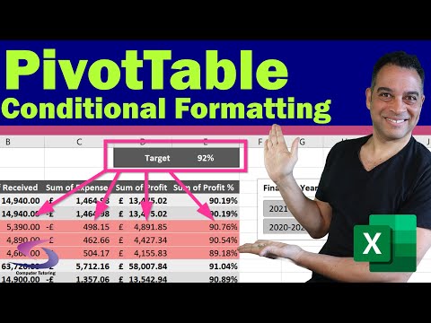
Pivot table conditional formatting can be used to change pivot table color formatting and highlight areas of interest in the pivot table. For example, in this video I show you how to highlight all loss making products with a red background.

One key issue with conditional formatting in PivotTables is that you can often end up including totals and subtotals when you don't want to. In order to apply conditional formatting to pivot tables you need to ensure you have selected the item type in the pivot table you want formatted. For example, select a subtotal for conditional formatting of pivot table subtotals, or select a main value to apply conditional formatting to pivot table values only.

When pivot table conditional formatting is not working it is often that the wrong option has been chosen, such as to only apply the format to the one value that happened to be selected at the time the formatting was applied. It can also look like pivot table conditional formatting disappears when this happens. this is dealt with in this video.

I want to show how you go about applying conditional formatting to pivot tables because one of the things that can go wrong straight away is it starts doing conditional formatting of subtotals. What really matters is where you start when you apply the conditional formatting, so which cell is highlighted. If I just happen to be on one of the subtotals and I apply conditional formatting, that will just do that one cell as things stand, but you'll see next to it you get this little icon here, and if you click down on here, apply formatting to, for example, all cells showing sum of sales. If you do that, you'll see that it includes the grand total. So the green number is obviously the grand total of everything which makes everything else look look quite bad. You can't really tell what's going on for it all. If I am on a normal number of any sort this one then excludes any totals as a genuine color grading or heat map of sales, which is much more likely to be what we're going after in the first place... so absolutely key you pick on the right thing before you start adding your conditional format.

In conclusion, mastering conditional formatting in Excel pivot tables empowers you to unlock valuable insights from your data with precision and clarity. By following these straightforward steps, you'll streamline your data analysis process and elevate the visual presentation of your reports. Remember to download the workbook for hands-on practice, and explore the possibilities of customized formatting to suit your specific needs. Keep honing your Excel skills to maximize efficiency and effectiveness in your tasks. Thanks for watching, and until next time, keep excelling!

[UpExcel]

✅ FREE Access to ALL Up4Excel Files. Includes Excel Templates, Training Workbooks, Example Data, Cheat Sheets and more. New Content Added Weekly!

[pupycron]

This is great. I never would have figured this out on my own. Thanks!

[wayneedmondson]

Thanks for the video. Some good tips there for getting started doing your Conditional Formatting from the right spot in the Pivot Table. Thumbs up!

[javierlp]

Hi!, is there a way to remove subtotals from only one column ?. I want the subtotal but not in all of them. Thank you

[rp]

But the formatting gets moved some rows down after I refresh the pivot table. Any ways around that?

[Scramblersj]

Hi . Can you color the 1st column based on formula ?

[UpExcel]

👉Conditional formatting on pivot tables is a little bit different to normal cells. In this video you will learn how conditional formatting can apply to totals, subtotals, and values independently...and how to switch between them ✅