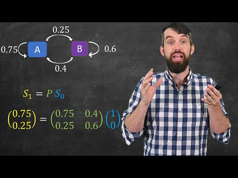
Introducing Markov Chains

A Markovian Journey through Statland [Markov chains probability
animation, stationary distribution]

[michelec]

I love all the little puns hidden in the video! (like the stamp from Bayesville)

[Annie-dbvh]

This is the best explanation I've seen so far. Thanks!

[barbaraulitsky]

This is such an amazing and hilarious video! It is easy to understand and super helpful. I absolutely love it!!! 😍🤩💖

[JoshCaiLovzu]

The more connected a city is, the more frequent it's visited. interesting finding!

[keegansayshi]

Thank you for explaining this to me like I'm a child.

[shaswatachowdhury]

So the important part is that, although there lies an inherent probability distribution of Anna's stay in cities based on the flight connectivity, Anna herself is not biased while taking her decision, i.e., to her all cities are equiprobable options.

So in Markov Chain Monte Carlo simulation (MCMC), X = {which city she will land for her next trip) is the random variable (parameter to be estimated in MCMC) whose value forms the Sample {X}, with E = {traveling to next destination} being the random event.
Now, starting from any point in the parameter space {Baysville, Averagemont, ...}, random walk biased by the underlying probability distribution (here, the probability of Anna's stay in different cities represented by the posterior of the parameter - city) is performed to obtain one Sample after another, (for example: {Baysville}, {Averagemont}, ...), where each sample is dependent on the previous one due to the Markovian nature of the process. The sequence of Samples {{Baysville}, {Averagemont}, ..., {Continuopolis}} forms the Markov Chain of length say 'n', containing transition from one city to the other for 'n' trips.
As we keep increasing the 'n', the random walk eventually converges to the equilibrium state, i.e., the probability of her stay in different cities does not change with increasing 'n' further.
Often, several Markov Chains are created in parallel with different starting points in the parameter space, to be absolutely sure of the convergence to the equilibrium state.
From the above, we get the probability distribution of her stay based in city. We can perform similar analysis where instead of city as parameter we chose the 'no. of connectivity' as the parameter; we will then get the probability distribution of her stay based on number of connectivities.
From these two probability distributions we can yield a correlation between the two set of parameters -- city and no. of connectivities.
Voila!

[yoto]

glad to found a hidden gem channel, love it!! 🥰

[RahmanHaghparast]

Really nice. Thanks for the great explanation.

[jokingz]

easy to understand and well explained. thank you!

[MrHenry]

wow thats really well explained, thank you!

[iurgnail]

would have been great if you showed whether the shape of connection network alone affects the result

[IwanAlqodrie]

the video is very useful and useful information, greetings success

[sanjaysg]

Just another average day at averagemont! I'm dead

[desaint]

Lmaooo the Cities are named after Math Concepts. Average, Continuous, Bayesian, Discrete, Vandermonde Matrix. Loll

[ElysonPanolino-gg]

simple topic get explained by complicated example 😢

[ViceKnIghtTA]

The 'Ana Markov' and 'Normal Distributors' company name was kind of distracting (you could have used any other random xyz or abc generic name). Otherwise a helpful video for beginners. Thanks.