Convert Text to Time Values with SUMPRODUCT (Data Cleansing Part 2)

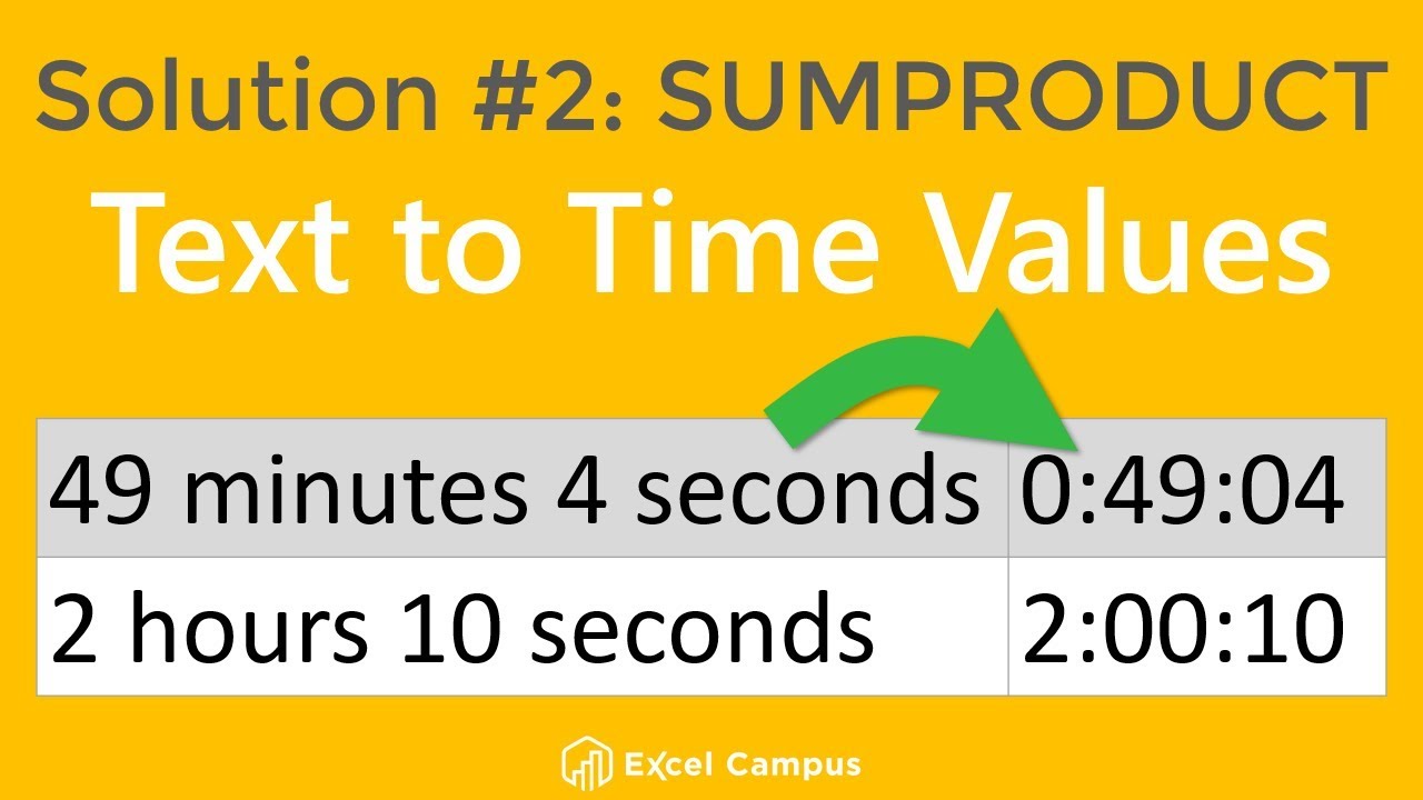
This is the second video in a series of solutions for our Data Cleansing Challenge. In this video I explain how to use a formula with SUMPRODUCT to convert the time stored as text into numeric time values in Excel.
Download the Excel file to follow along:

This allows us to convert all the time increments (hours, minutes, seconds) into seconds within a single formula. We then divide by the total number of seconds in a day to return the time value.

In the video I walk through writing the formula.

You will learn how to use an array (list) of values within SUMPRODUCT. We can feed the search function multiple values to extract time period.

The array of values are listed in curly brackets.

{"h","m","sec"}

I also explain how the SUMPRODUCT function calculates these arrays by multiplying the items together and then summing them up.

00:00 Introduction
01:55 SUMPRODUCT Function
09:39 SUMPRODUCT Explanation
11:10 Convert Text to Time

[philchua]

FINALLY!!! I have been racking my brains for WEEKS on how to do this without helper columns. Thank you, Thank you!, THNAK YOU!

[ahmedJaber]

thank you for sharing this formula. I love it. it is one of the very few techniques i have seen in the past many years that got me excited.

[katerina]

Thank you so much John, complex and very clear, looking forward to the next video

[vigneshwarank]

Jon, the explanation for sumproduct function is awesome.
I want to say that sumproduct is the greatest function, I have ever used . It has reduced my weeks of work into few minutes.
I expecting you to make a separate detailed video on sumproduct function.

[umehtoch]

Great trick there. Looks easy but complex. Thanks for educating me once again

[wayneedmondson]

Hi Jon.. cool solution using SUMPRODUCT. Thanks for sharing it. Also, for your first solution using TEXT functions, you can use the padding zero / 0& trick shown in this solution to eliminate the MAX function.. as in.. =IFERROR(VALUE(MID(0&$C2, SEARCH(I$1, 0&$C2)-3, 2)), 0). Great to learn all these innovative techniques for solving the same problem. Thumbs up!
PS - Also, I discovered that the TIME function is smart enough to convert TEXT numerals into values. So, the VALUE function is not needed. This formula works as the input to the TIME function: =IFERROR(MID(0&$C2, SEARCH(I$1, 0&$C2)-3, 2), 0).. conversion to VALUE is not required.. TIME does it automatically.

[CCrider]

This was a very informative video. I just happen to be learning how to formulate times on eRouters for lab products and this may have just made my life a bit easier.  Thank

[charleszema]

This is fantastic, but I am getting data from a vendor as: 1d 3h 13m 1s. What is your suggestion to get to time 00:00:00?

[SimonTidd]

Hey Jon, What do you do in this option, or the more simple text formulae first video options, with durations of three digits e.g. "120 hours"? I've not had a go but would the combination of MID, SEARCH/FIND and the -3 characters cause problems with the fixed 3 being the culprit? I am not sure how I'd work around that. Any ideas?

[Rkeev]

Can sumproduct subtract col a from column b, but only sum the numbers where the results of the subtraction are greater than zero?

[kakularsrikanth]

Hi, can you plz convert this "2 days 23 hours 59 minutes" hours and "HH:MM" format

[williamarthur]

Well that was great, no way would I have come up with it, still not sure about the zero padding, will have to look closely to see how it works. Mind you I'd never thought of dividing by 86400, I've just alway gone; / 60 wrap it and /1440 .