How To Create Dynamic Dependent Drop Down in Google Sheet for Every Row ? ! Best and Easiest Method

#dropdownlist
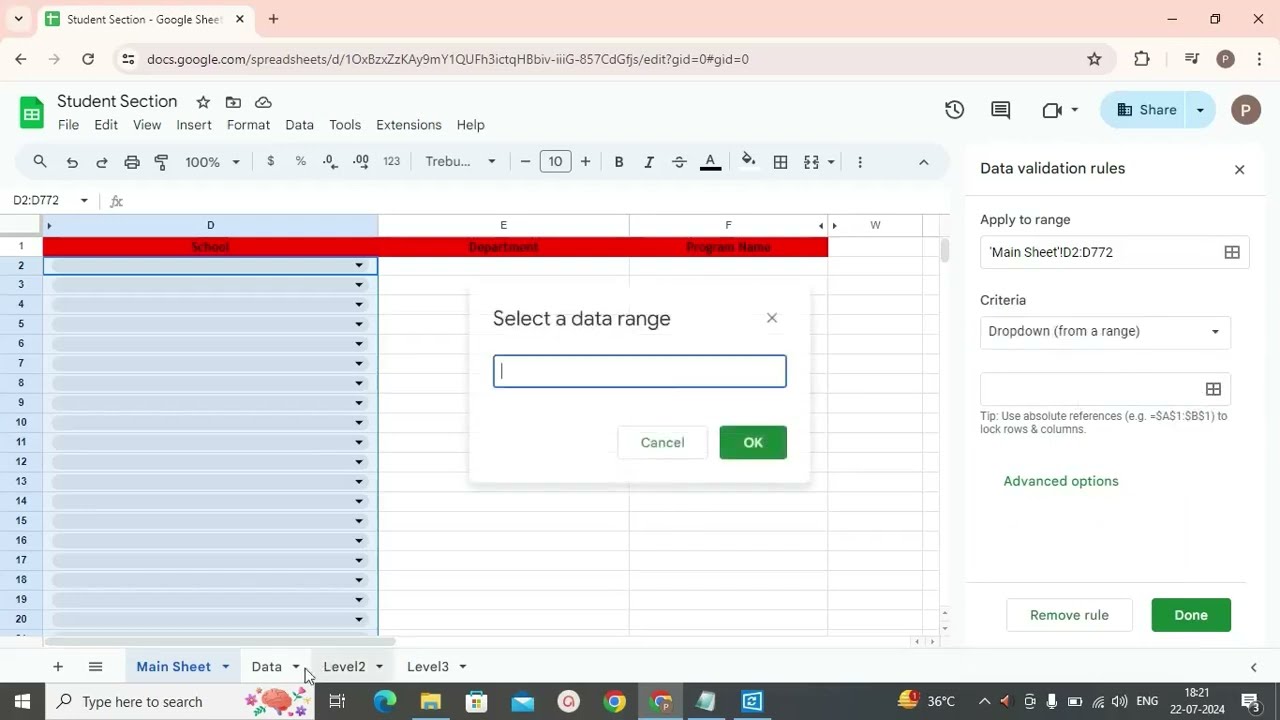
Creating a dynamic dropdown in Google Sheets for every row typically involves using a combination of named ranges and data validation. Here’s a step-by-step method to achieve this:

### Step-by-Step Guide

1. **Prepare Your Data**:
- Ensure you have your list of options prepared. For example, if each row needs a dropdown with different options, have these options listed somewhere in your sheet.

2. **Set Up Named Ranges**:
- Go to **Data Named ranges** from the top menu.
- Click on **Add a range**.
- Define a named range for each row where you want a dropdown. For example, if your data starts in column B and you have multiple rows, name the ranges like `Dropdown1`, `Dropdown2`, etc. Each range should cover all the options for a particular row.

3. **Apply Data Validation**:
- Select the cell or range where you want the dropdown to appear for each row.
- Go to **Data Data validation** from the top menu.
- In the criteria section:
- Choose **List of items**.
- Enter the formula `=INDIRECT("Dropdown"&ROW())` for the **Criteria range**. This formula dynamically selects the named range based on the current row number.
- Make sure to select **Cell range** and specify the range where you want the dropdown to appear.

4. **Test Your Dropdowns**:
- Now, when you enter data into each row, the dropdown list will dynamically adjust based on the named range associated with that row.

### Example

Let’s say you have a Google Sheet where:
- Column A has different categories.
- Column B needs a dropdown based on the category in the same row.

- **Step 1**: Suppose you have your options listed in separate columns (e.g., C, D, E for each row).
- **Step 2**: Name each range (e.g., `Dropdown1` for row 1, `Dropdown2` for row 2, etc.).
- **Step 3**: Apply data validation to each cell in column B, with the criteria `=INDIRECT("Dropdown"&ROW())`.

This setup ensures that each row in column B will have a dropdown list dynamically populated based on the category chosen in column A.

### Notes

- **Updating Options**: If your options change frequently, update the named ranges accordingly.
- **Managing Large Data**: For large datasets, consider using Apps Script for more automated and scalable solutions.

By following these steps, you can create dynamic dropdowns in Google Sheets that adjust for every row based on your specified criteria.