filmov
tv
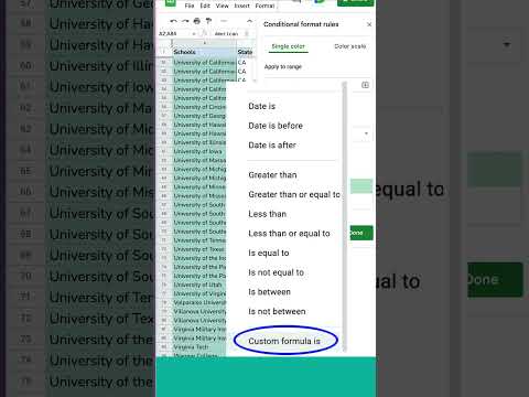
How to color duplicates from two columns in excel #exceltips

Показать описание
You can use conditional formatting in Excel to highlight duplicate values between two columns. Here are the steps:
Select the two columns that you want to compare for duplicates.
Click on the "Home" tab in the Excel ribbon.
Click on the "Conditional Formatting" button in the "Styles" section.
Choose "Highlight Cells Rules" and then "Duplicate Values" from the drop-down menu.
In the "Duplicate Values" dialog box, select "Duplicate" in the "Values" section.
In the "Format" section, choose the formatting you want to apply to the duplicate values. For example, you could choose to highlight them in red.
Click "OK" to close the dialog box and apply the conditional formatting to the selected cells.
Now, any duplicates between the two columns will be highlighted according to the formatting you chose.
how to find duplicates in excel,find duplicates in excel,highlight duplicates in excel,colour duplicate values in excel,how to compare two columns in excel,how to compare two columns in excel using vlookup,microsoft excel,how to remove duplicates in excel,excel,how to highlight duplicates in excel,excel highlight duplicate values in different colors,remove duplicates in excel,compare two columns in excel,compare two lists in excel for matches
 0:00:29
How to highlight duplicate values in Excel! #excel #exceltips #exceltutorial
 0:00:27
Find duplicates from two separate lists in Excel with Conditional Formatting! #excel #exceltips
 0:03:48
How to Highlight Duplicates in Excel (Super Easy)
 0:08:40
How to Find Duplicates in Excel & Highlight Duplicates If You Need To
 0:00:16
Excel Trick: Highlight Duplicate Entries with Ease | Conditional Formatting | Excel Shorts
 0:00:30
Highlight Duplicates in Google Sheets SHORTS || Use Conditional Formatting to Find Duplicates
 0:02:07
Google Sheets - Highlight Duplicate Data in a Column or Row
 0:00:25
Highlight & Remove Duplicates in excel
 0:01:00
How to Highlight Duplicate Values in Google Sheets
 0:00:48
How to find duplicates in Google Sheets
 0:05:25
Highlight Duplicates in Excel in Same Column in a Different Colour
 0:00:49
Highlight Duplicate Values in Google Sheets #shorts
 0:01:23
How to color duplicates from two columns in excel #exceltips
 0:05:56
Compare Two Excel Worksheets & Find Duplicates Using Formula or Conditional Formatting
 0:00:31
How To Highlight Duplicate Values with Red Color in Excel? |excel tips | #excel #shorts #viral
 0:06:47
Excel - Find & Highlight Duplicate Rows - 3 Methods | Conditional Formatting
 0:03:36
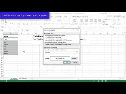
Excel - Conditional Formatting find duplicates on two worksheets by Chris Menard
 0:02:25
How To Highlight Duplicates in excel | Conditional Formatting in Excel Color coding | #msexcel
 0:00:31
How to Highlight Duplicate Values Except First Instance in Excel? #shorts
 0:03:00
How to Highlight Duplicates in Google Sheets
 0:09:43
Compare Two Sheets for Duplicates with Conditional Formatting
 0:00:51
How to Highlight Duplicates with Different colors in Excel sheet
 0:04:00
How To Filter For Duplicates Using Conditional Formatting In Excel
 0:00:29
How to identify duplicates in excel #chanzify #excel #exceltips #duplicates
Комментарии