filmov
tv
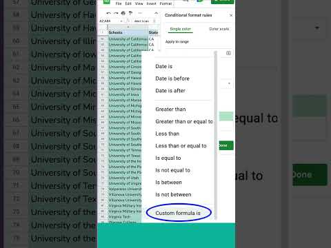
Google Sheets - Highlight Duplicate Data in a Column or Row

Показать описание
Learn how to use conditional formatting in Google Sheets to highlight cells with duplicate data.
To do a row instead of a column, use 1:1 to reference all of row 1, just like you use A:A to reference all of column A.
If you live in a country that uses a comma as a decimal separator, use semi-colons instead of commas.
Learn more from Prolific Oaktree:
#googlesheets #spreadsheets #duplicates
To do a row instead of a column, use 1:1 to reference all of row 1, just like you use A:A to reference all of column A.
If you live in a country that uses a comma as a decimal separator, use semi-colons instead of commas.
Learn more from Prolific Oaktree:
#googlesheets #spreadsheets #duplicates
 0:02:07
Google Sheets - Highlight Duplicate Data in a Column or Row
 0:00:48
How to find duplicates in Google Sheets
 0:05:06
HOW TO FIND DUPLICATES IN GOOGLE SHEETS | Finding and Highlighting Duplicates in Google Sheets
 0:00:30
Highlight Duplicates in Google Sheets SHORTS || Use Conditional Formatting to Find Duplicates
 0:02:54
How to Find Duplicate Values in Google Sheets
 0:03:00
How to Highlight Duplicates in Google Sheets
 0:00:57
How to highlight duplicates in google sheets 2024 (Quick & Easy)
 0:01:59
How to Highlight Duplicates in Google Sheets
 0:08:21
How to Highlight Duplicate Values in Google Sheets | Highlight Duplicate Data in a Column or Row
 0:04:22
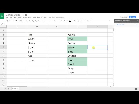
Google Sheets - Compare Two Lists for Matches or Differences
 0:19:40
Google Sheets - Conditional Formatting Duplicate Values Tutorial - Highlight Duplicates
 0:02:57
How to Find and Remove Duplicates in Google Sheets
 0:13:31
Google Sheets - 6 Ways to Highlight Duplicates ✅❌| Conditional Formatting Custom Formula | COUNTIF...
 0:05:06
Google Sheets - Highlight Duplicate Data using Conditional Format (updated 2021)
 0:04:15
Google Sheets - Identify Duplicates between Two Worksheets
 0:05:20
Highlight Duplicate Values and Extract Unique Values in Google Sheets
 0:06:32
Highlight Duplicates in Google Sheets: Real-World Examples
 0:01:07
How To Highlight Duplicate Rows in Google Sheets
 0:01:32
Google Sheets Tutorial - Highlight Duplicate Data in a Column or Row
 0:04:18
Google Sheets - Highlight Duplicates In Google Sheets | Highlight Duplicate Data In A Column Or Row
 0:01:00
How to Highlight Duplicate Values in Google Sheets
 0:09:29
Highlight Duplicates in Google Sheets - Malayalam Tutorial
 0:00:30
How to Highlight Duplicates in Google Sheets | #shorts #google #googlesheets
 0:01:32
How to highlight duplicates in Google Sheets
Комментарии