Basic Excel Business Analytics #41: Excel 2016: Introduction to PowerPivot & Data Model

Learn about PowerPivot & Data Model in Excel 2016.
1) (00:11) Intro to what we will do in this video
2) (00:30) Step 1 for Building Data Model: Get Data into PowerPivot. For our example we convert Proper Data Sets in Excel to a Table and use “Add to Data Model” button in PowerPivot Ribbon Tab
3) (01:00) Excel 2016: New PowerPivot Ribbon Tab. They have renamed “Calculated Field” Button (Excel 2013) to “Measure” button (Excel 2016). We can build DAX Measures (Calculated Fields) with this new button.
4) (02:24) Step 2 for Building Data Model: Create Relationships between related tables using the “Diagram View” button in the “Manage Data Model” window.
5) (02:47) Excel 2016: New one-to-many visual presentation in the Diagram View window. We can see a line with the number one ( 1 ) next to the primary key field in the lookup table (dimension table) and an asterisk next to the Foreign Key in the Fact table.
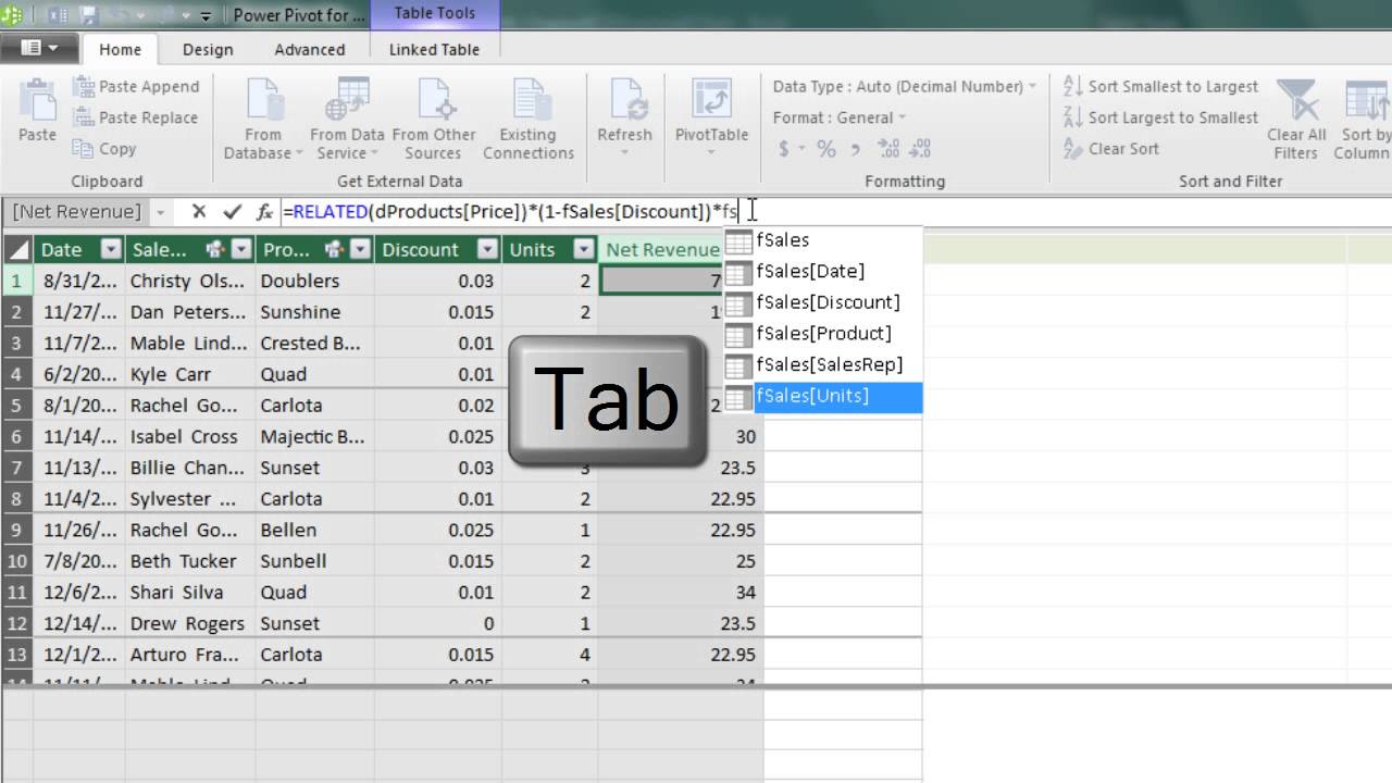
6) (03:34) Step 3 for Building Data Model: Build DAX Calculated Column formulas. In this example we calculate Net Revenue for each transaction using the RELATED DAX function and the ROUND DAX function and a number of columns from the Fact Table. We also learn about the convention for adding columns to DAX formulas: ALWAYS use the Table Name and the Field Name (Column Name) with square brackets around it.
7) (05:56) Discussion of Implicit vs. Explicit formulas.
8) (05:56) Step 3 for Building Data Model: Build DAX Measures (Calculated Fields) formulas. In this example we will calculate Total Net Revenue using the DAX SUM function and the Calculated Column from our Fact Table. This is an explicit formula that can work efficiently with the Columnar database on big data sets.
9) (07:17) Add Number Formatting to Measure (Calculated Field)
10) (07:32) Discussion of Filter Context: The ability of the Measure (Calculate Field) to respect criteria in the PivotTable and filter the underlying table to result in a range that is smaller than the full table size and will contribute to faster formula calculation time; in essence the DAX formula and the Columnar Database work together efficiently – and much more efficiently than normal PivotTable calculations or normal spreadsheet Excel formulas.
11) (08:00) Build PivotTable from Data Model
12) (08:30) Excel 2016: New “F of X” Function Icon for Measures (Calculated Fields) in the PivotTable Field List.
13) (09:23) More discussion of Filter Context and why DAX Measures (Calculated Fields) can calculate efficiently on Big Data.
14) (09:59) Summary and Conclusion
Download Excel File Not: After clicking on link, Use Ctrl + F (Find) and search for “Highline BI 348 Class” or for the file name as seen at the beginning of the video.
Introduction to PowerPivot and Data Model in Excel 2016, What is PowerPivot Excel 2016? What is Data Model Excel 2016? What is New in Excel 2016 PowerPivot? What is new in Excel 2016 Data Model?

[shubhampawar]

❤️👌 It's my dream to meet you, Sir 😊

[caseydonnell]

These are far away the best overviews of the new options in Excel 2016, that I have found so far.

[wasimbader]

thank you again, I have a written a lot in video or tutorial 42. thumbs up. You are doing a great job, for being a teacher a big respect from my heart. Regards

[pmsocho]

The dropdowns with function names, table names, field names and measure names are so cool in Power Pivot. I wish it would be implemented in Power Query also because case sensitive functions in Power Query drive me crazy :)

[christhomas]

Well presented and really useful, thank you

[szetinglam]

Thank you for the great video! I would like to ask is it possible to use if functions in power pivot measure formulae? Thank you:)

[chrisbohan]

I am having a problem setting my OLAP drill through limit higher than the default. Using Excel 2016 and PowerPivot. When I go to Data>Connections>Properties (for "ThisWorkbookDataModel") and change the OLAP Drill Through Maximum number above 1000,  I receive this error... "This connection name is already in use. Try a different name" I am using big data and frequently I need to have as many as the first million rows returned in my drill through. Anything I changed in 2013 (before the upgrade) has stayed at the million row mark, but anything new I cannot change.

[andyy]

Beginner to Power Pivot~ One quick question: How can I create a linked table in power pivot using Excel 365? There is no even a Linked Table ribbon at the top...

[brettittersagen]

Beginner to Power Pivot - Why wouldn't one just use a vlookup or a index(match) to get the 3 tables together?