Excel Magic Trick 1444: Logical Formulas: Count & Extract Customer Names for 8 Sales Coupon Groups

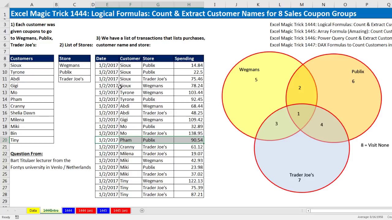
See how to use Excel Formulas to analyze a group of customers who have been given coupons to three stores. Our goal is to count how many customers used coupons in one of eight coupon groups (all combinations of the three store coupons) and then extract the customer names in each group. The data and goals are:
1) Each customer was given coupons to go to Wegmans, Publix, Trader Joe's.
2) We have a list of Stores names.
3) We have a list of transactions for the coupon redemptions that lists purchases, customer name and store
4) Goal 1: Count Customers who visited a given set of stores.
5) Goal 2: List Customers who visited a given set of stores.

Topics in Video:
1. (00:12) Introduction to Problem
2. (03:33) Count number of coupons each customer redeemed for each store. See the COUNTIFS Function.
3. (07:03) Logical formulas for determining which customers fall into each of the eight coupon groups. Learn about AND Logical Tests, OR Logical Tests, and a NONE Logical Test (None are TRUE, or All are FALSE). See the Excel Spreadsheet Logical functions: AND, OR, NOT.
4. (17:23) Count Customers in each of the eight coupon groups using COUNTIFS Function.
5. (18:02) Formula to Extract Customer Names for each of the eight coupon groups. Learn about Array Formulas to looks an item and Return Multiple Items. Learn about the Excel Spreadsheet functions: ROW, AGGREGATE, ROWS, INDEX and IF.
6. (29:25) Conclusion

Related Videos:
Excel Magic Trick 1444: Logical Formulas: Count & Extract Customer Names for 8 Sales Coupon Groups
Excel Magic Trick 1444 Part 2: Count Customer Names for 8 Sales Coupon Groups
Excel Magic Trick 1445: Single Cell Array Formula: Count Customer Names for 8 Sales Coupon Groups
Excel Magic Trick 1446: Power Query Count & Extract Customer Names for 8 Sales Coupon Groups
Excel Magic Trick 1447: DAX Formulas & Data Model PivotTable to Count & List Stores Customers Visited

[LeilaGharani]

I really like your NOT-OR combination - smart approach! Thank you for the logical tests and aggregate fun :)

[mahamohan]

Its always a fun to learn from the wonderful master teacher

[BillSzysz]

Remarkable video!!
Give Mike a problem and see what a fantastic solution it will find. He will solves everything !!! :-)))
Thanks Mike !!!

[MySpreadsheetLab]

I like how you used the AND function. thanks for the video Mike!

[barttitulaerexcelbart]

Mike, amazing video. The nesting of so many different formula's in one cell, and then, so logically explained. It is absolutely recommendable to watch your video's. What is tippical for Excel is that there are always more ways to accomplish, Excel ninja's know more ways to do someting, but they also know WHY. I like it that you also explain (not only in this video but always) the pro's and con's of every Excel way of doing things. Thanks Mike !!

[ndelpurg]

MANY THANKS for all your great teaching videos -

[mohamedchakroun]

Thanks Mike for what you are doing this is an example of the power of the excel formulas i love it

[brianjensvold]

I like it! If I was faced with this problem I would have just identified which group each person belonged to in column N using a admittedly large nested IF statement, then make a pivot table from that.

[jerrydellasala]

The new FILTER function makes the "List Customers who visited a given set of stores." really easy! The formula in the top right corner of the result table is
=FILTER($J$9:$J$20, O9:O20)
The results spill down and the formula can just be copied across. SWEET!
That filters the list of customers ($J$9:$J$20) by the TRUE/FALSE Group columns (O9:O20). The group columns (O9:O20) don't need to be locked in either direction since the formula only appears in the top column - the rows aren't referenced across the columns, and the columns do need to be relative.
The same is true for the table of Customers belonging to each of the 8 groups on the Data worksheet starting in cell X12. [=FILTER($I$13:$I$1012, O13:O1012)]

[lessnyder]

Another great video, thanks for all the awesome tips you've shared through the years!

[vida]

Interesting solution for interesting task. Waiting for upcoming videos

[rockguitarist]

Fantastic instruction Mike! I thought we'd be using Match, but you came up with a totally awesome solution!

[willwright]

Great video as always, Mike. For future reference, note that the grocery store Wegmans is pronounced like "LEG-mans."

[warnford]

Excellent viddies Many thanks - following your Highline Business course and found it very useful
Can I pick ?Sioux and Miki have gone to all three (1.05) - but the intersecting circles WUPUT ( using obvious notation) only has a one in it and not a two

[rajkumarrajan]

I want to do it for a large data set 30 columns and around 75000 rows
will it work without glitch

[Goval]

Hey bro, love your vids! I've learned so much..

I have a problem and I would like to see your approach to it.

At work I'm receiving 2 reports with investment accounts, financial advisor name, quantity invested and sector. One report is old and the other is the new one they are testing and they want me to identify the unique transactions between both reports. I've been doing it with conditional formatting and creating an unique ID using concatenate, but when the data set is TOO BIG is almost impossible since the computer slows down too much.

after conditional formatting highlights the unique accounts I go back to each report and start searching one by one with the filter.

Is there another way of doing this??

thank you! I'm pretty sure a video of this would really help others as well.