filmov
tv
How to search value and auto highlight row in excel @BrainUpp

Показать описание
Highlight Rows Based on a Text Criteria
Select the entire dataset (A2:F17 in this example).
Click the Home tab.
In the Styles group, click on Conditional Formatting.
Click on 'New Rules'.
In the 'New Formatting Rule' dialog box, click on 'Use a formula to determine which cells to format'.
Search and Highlight Data Using Conditional Formatting
If you work with large datasets, there can be a need to create a search functionality that allows you to quickly highlight cells/rows for the searched term.
While there is no direct way to do this in Excel, you can create search functionality using Conditional Formatting.
For example, suppose you have a dataset as shown below (in the image). It has columns for Product Name, Sales Rep, and Country.
Now you can use conditional formatting to search for a keyword (by entering it in cell C2) and highlight all the cells that have that keyword.
Something as shown below (where I enter the item name in cell B2 and press Enter, the entire row gets highlighted):
In this tutorial, I will show you how to create this search and highlight functionality in Excel.
Later in the tutorial, we will go a bit advanced and see how to make it dynamic (so that it highlights while you’re typing in the search box).
Search and Highlight Matching Cells
In this section. I will show you how to search and highlight only the matching cells in a dataset.
Here are the steps to search and highlight all the cells that have the matching text:
Select the dataset on which you want to apply Conditional Formatting (A4:F19 in this example).
Click the Home tab
In the Styles group, click on Conditional Formatting.
In the drop-down options, click on New Rule.
In the ‘New Formatting Rule’ dialog box, click on the option ‘Use a formula to determine which cells to format’.
Enter the following formula: =A4=$B$1
Click on ‘Format..’ button
Specify the formatting (to highlight cells that match the searched keyword)
Click OK.
Now type anything in cell B1 and press enter. It will highlight the matching cells in the dataset that contain the keyword in B1.
How does this work?
Conditional Formatting gets applied whenever the formula specified in it returns TRUE.
In the above example, we check each cell using the formula =A4=$B$1
Conditional Formatting checks each cell and verifies it the content in the cell is the same as that in cell B1. If it’s the same, the formula returns TRUE and the cell gets highlighted. If it isn’t the same, the formula returns FALSE and nothing happens.
Search and Highlight Rows with Matching Data
If you want to highlight the entire row instead of just the matching cells, you can do that by tweaking the formula a little.
Below is an example where the entire row gets highlighted if the product type matches the one in cell B1.
Here are the steps to search and highlight the entire row:
Select the dataset on which you want to apply Conditional Formatting (A4:F19 in this example).
Click the Home tab.
In the Styles group, click on Conditional Formatting.
In the drop-down options, click on New Rule.
In the ‘New Formatting Rule’ dialog box, click on the option ‘Use a formula to determine which cells to format’.
Enter the following formula: =$B4=$B$1
Click on ‘Format..’ button.
Specify the formatting (to highlight cells that match the searched keyword).
Click OK.
The above steps would search for the specified item in the dataset, and if it finds the matching item, it will highlight the entire row.
Note that this will only check for the item column. If you enter a Sales Rep name here, it will not work. If you want it to work for Sales Rep name, you need to change the formula to =$C4=$B$1
Note: The reason it highlights the entire row and not just the matching cell is that we have used a $ sign before the column reference ($B4). Now when conditional formatting analyzes cells in a row, it checks whether the value in column B of that row is equal to the value in cell B1. So even when it’s analyzing A4 or B4 or C4 and so on, it’s checking for B4 value only (as we have locked column B by using the dollar sign).
Related searches
How to highlight entire row in Excel with conditional formatting
excel highlight row shortcut
highlight row based on cell value google sheets
highlight active row and column
how to use conditional formatting in excel
conditional formatting row
highlight rows based on cell value
 0:01:58
How To Search Value In All Open Excel Workbooks?
 0:01:00
MS Excel LOOKUP Formula: Return Multiple Values
 0:00:59
How to search value and auto highlight row in excel @BrainUpp
 0:00:12
Excel tip advanced filter unique values
 0:00:48
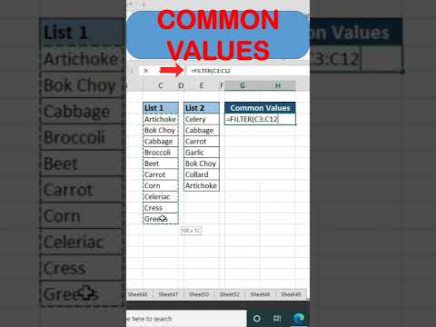
Find the Common Values between two lists in Excel using FILTER Function in Excel 365/Excel 2021
 0:00:29
Search Function in Excel Excel Trick Formula Shortcut Keys #shorts #youtubeshorts #excel #viral
 0:00:46
How To Search For A Value And Highlight The Row Automatically In Excel #dataanalysis
 0:00:39
Find Common Values From Two List In Excel @BrainUpp
 0:50:56
Seamless Search in Action: Drive Incremental Value Across Your Search Strategy
 0:02:58
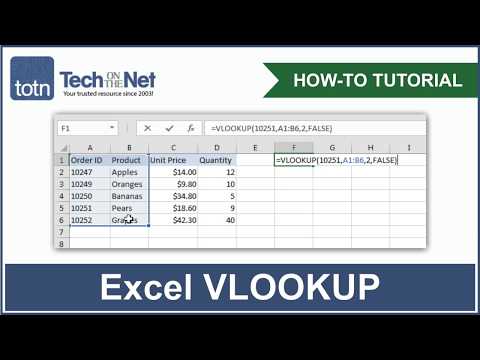
How to use the VLOOKUP function in Excel
 0:00:58
How To Find Your Purpose – Ikigai
 0:00:31
How to compare two lists to find missing values in excel - Excel Tips and Tricks
 0:06:59
How to Search Value Number from Array in Java Netbeans
 0:00:36
Easily compare two Excel lists for duplicates or unique values
 0:00:30
How To Find The Highest Number In Excel function @Brain Up
 0:00:46
How to search value and auto highlight row in MS Excel #Excelwithsonal
 0:05:31
Google Sheets: vlookup to search for a value in another range and return a corresponding value
 0:06:01
How to search keys for a value in dictionary
 0:00:18
Count Distinct Values in 10 Seconds Using Excel! 💪🏼 #excel
 0:04:11
How to Search Value in All Excel Files in a Folder Using Excel
 0:03:03
How to activate the 'RAID SEARCH VALUE' option - Arena Breakout
 0:14:34
VBA to Search Value on Multiple Sheets
 0:05:08
How to search for a value in Excel and return the number next to it.
 0:00:25
Use the countif function to find out how many times something comes up in a table. #excel #countif
Комментарии