Conditional Formatting with Two Conditions - Excel Tip

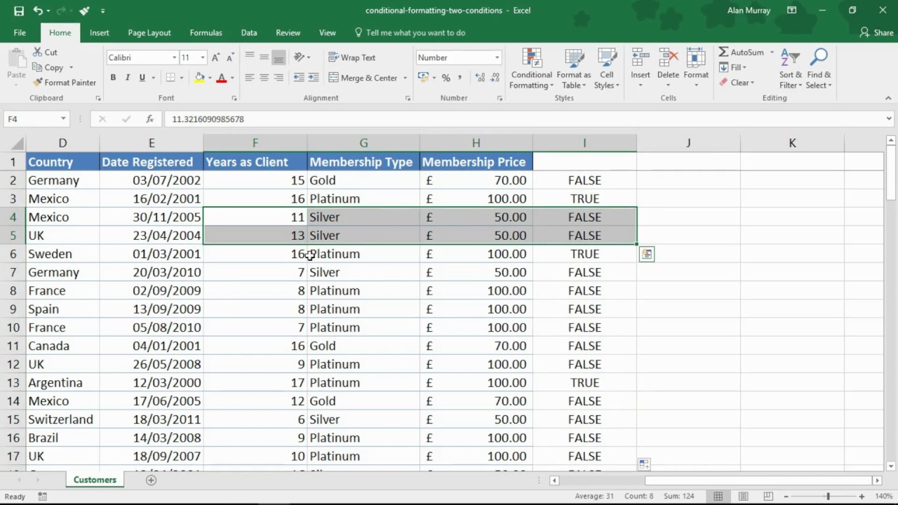
This video tutorial will show you how to use Conditional Formatting with two conditions. In the video will write a formula to test two columns and then apply the Conditional Formatting to an entire row.

Using the skills learnt in this tutorial you will know how to test multiple conditions in a Conditional Formatting rule, beyond just two conditions.

Find more great free tutorials at;

*** Online Excel Courses ***

Connect with us!

[trudifitzsimmons]

Thanks, saved me hours of playing around :)

[gopalakrishnarao]

Thanks a lot, for your informative video.

[antoniobacic]

Too good, thank you so much!
PS if specific gridlines can be automatically highlighted (for example 0 in a chart containing positive and negative numbers) that would be awesome if you also show.
Thank you.

[vishalshinde]

Thank you very much. Explained very nicely in short and simple way.

[SanjayKumar-yxgc]

It was interesting formula. I am waiting for your next video to use condition formatting. Thx a lot.

[StellaSaliu]

Nice video.
Could you clarify, what is the problem with Formula:
=and($F2<=TODAY(), $I2="Done")

Excel does not recognize the formula, but everything seems to be ok

[nya___nya]

Thank you sir. You helped me so much in my home work.

[ksanymilar]

How to conditional formatting by comparing dates on 2 different columns & with conditions on 3rd column?

[TheNuclearPhysician]

I have been searching for this method for months now. And now I found it.


Three cheers to you sir.

[jjeennssoonn]

Hi - How would i do multiple colour? ie Platinum can be green, Gold can be yellow and silver can be blue?

[mohammadmoinulhaquethakur]

I wish to calculate like:
Cell1: lets guess that there is a total amount of money in cell 1.
Cell2:- if Cell 1 is more or equal to then show only if less than then show the subtract amount.
Cell3:- if Cell 1 – cell 2 is more or equal to then show only if less than then show only subtract amount.
Cell4:- subtract amount of Cell1 – (cell 2 + cell 3)

[visionmachineryinc.]

First of all, your videos have been so helpful so thank you! Secondly, question. If I wanted to do conditional formatting with two conditions and one of those conditions is not a value it's either blank or not blank (but the content will vary), I thought I would put "*" to reference if there is or isn't something in the cell. Is there something else I would need to put instead?

[chanchalchanani]

not able to use this formula in office 2013. Please help

[atnenwynu]

This was a huge time saver for me :) Thank you for the tutorial!

[Moonlightkitteh]

Thank you! Time to impress the office again :D

[zumazmusic]

Right on, this helped me accomplish my goal! Cheers from Los Angeles.

[Shippersmallcom]

Perfect! And it was the first video I found too! Must be my day! Thanks for the tutorial Mate! I subscribed and saved this in my tech tutorials folder.

[thewanderboyjitinraj]

can we apply different conditional formatting for data in rows and columns?

[hemantsharma]

if in a sheet having three coloum 1st containing easy, medium, diffcult in continues manner, 2nd containing wrong, right,blank in continues manner, in 3rd coloum having topic name how to print topic name of blank and wrong questions using easy, medium, hard colum

[Gyongyver]

Hi, how would the formula look like if you had (1) Platinum, (2) Silver, (3) Gold, (4) Bronze, (5) Diamond and (6) Basic memberships and you want to highlight the following memberships over 10 years? (1) Platinum, (2) Silver, (3) Gold. Thanks a lot :)