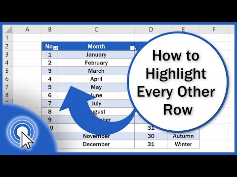
Alternate Row Color with Conditional Formatting in Excel

A great Excel trick to alternate row color using Conditional formatting.

Steps:
1. Highlight range

2. Alt + H + L + R to bring up Conditional Formatting menu

3. Create new rule

4. Click "use a formula to determine which cells to format."

5. Type =MOD(ROW(),2)=1

6. Format however you'd like (I chose gray shading in the video)

7. Click OK a bunch of times

That's it! Now your row color alternates in the range. Great for dashboards and other outputs.

A couple ways to get to know me better⤵️

Thanks for watching!
—Chris

[jeffsirkis]

This is much easier than methods I’ve used in the past. Thanks!

[BurksAustin]

That’s awesome, thanks! I used to do this with a helper column and SEQUENCE, but will switch to this for sure

[hexmech]

Don't use this with merged tables. I found out that it doesn't color everything properly.