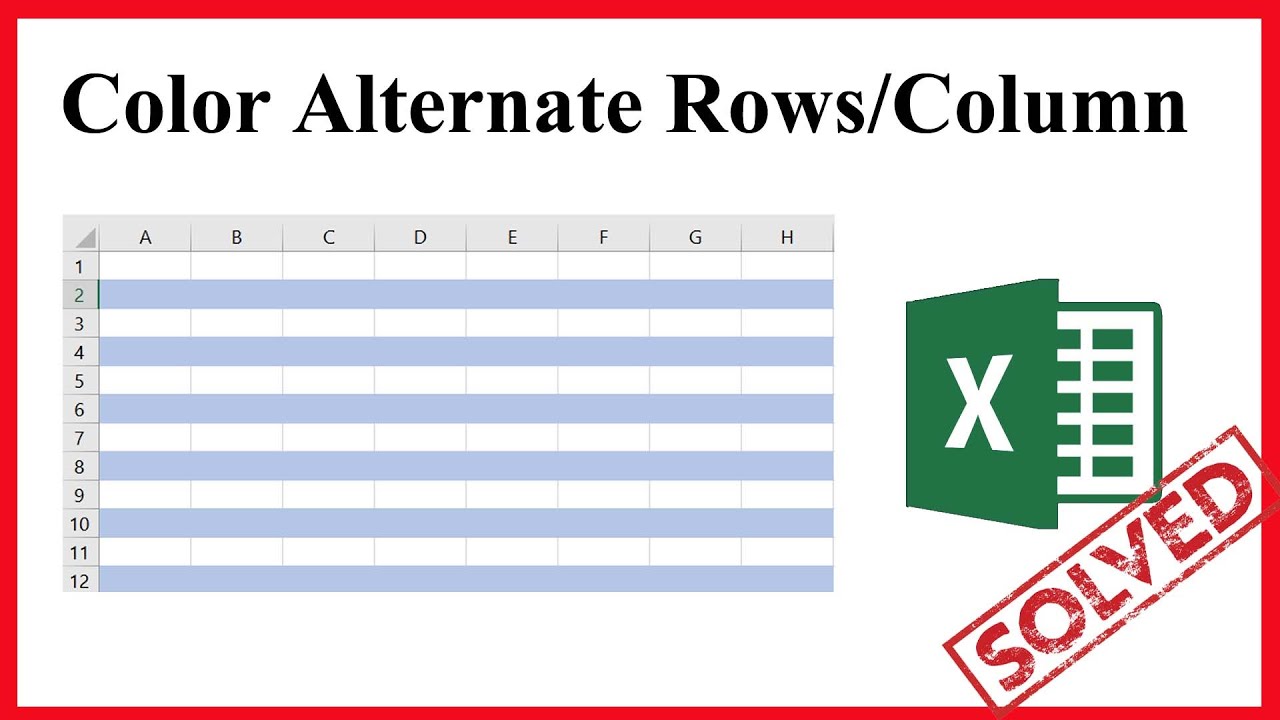
How to apply color banded rows or columns in excel

How to apply color banded rows or columns on excel or how you can color or shade every alternate rows or columns in excel. Yes. This is what you are going to learn today. Welcome to excel 10 tutorial and lets get started.

Color Banded Rows: Color banded rows indicate every second/alternate rows with color/shading.To attain this you'll have to use conditional formatting. Lets follow the below procedure to color every alternate rows.

Step 1: Select the cell ranges where you want to apply color.
Step 2: In the home tab click on conditional formatting.
Step 3: Select "New Rule"
Step 4: Select "Use formula to determine which cells to format"
Step 5: Paste this formula in the formula bar for coloring every alternate rows.
=MOD(ROW(),2)=0
Step 6: Click "Format" and select "Fill"
Step 7: Select the color and click ok and ok again.
Done you have successfully color banded excel rows.

Color Banded Columns: Color banded columns indicate every second/alternate columns with color/shading.To attain this you'll have to use conditional formatting. Lets follow the below procedure to color every alternate columns.

Step 1: Select the cell ranges where you want to apply color.
Step 2: In the home tab click on conditional formatting.
Step 3: Select "New Rule"
Step 4: Select "Use formula to determine which cells to format"
Step 5: Paste this formula in the formula bar for coloring every alternate columns.
=MOD(COLUMN(),2)=0

Step 6: Click "Format" and select "Fill"
Step 7: Select the color and click ok and ok again.
Done you have successfully color banded excel columns.

Thanks for watching.
#Color #AlternateRow
-------------------------------------------------------------------------------------------------------------
Support the channel with as low as $5
-------------------------------------------------------------------------------------------------------------
Please subscribe to #excel10tutorial

Playlists:

Social media:

[SVCmusic]

You are a genius. Excel couldn't give these simple instructions and after a half hour of looking, boom. Your instructions worked like a charm. Also, thank you for putting the instructions in the information because I am a bit of an impatient person and just wanted a step by step written out but I left the window open so your video played fully in case you are monetized.

[mohsenshayan]

I like it when a good YouTuber like you shows the end result at the beginning of their video. I subscribed you just when I saw this.

[remski]

If only I could like this video 10K times.. thank you so much for sharing your knowledge. You earned new subscriber!

[alisalis]

Excellent video, the best on this topic thus far. Thxs so much!

[sadimohammad]

No trash talk. I like it.
Thumbs up.

[andrescastro]

Thank you, straight to the point. done thanks again

[anuaugustin]

This was really helpful today. Thanks :)

[shiwanisaini]

💯 it's work good. My problem is solve. Thank so much. 😇

[SameBet]

Can you do a video that would show us how to band 2 rows? For example, rows 2 and 3 would be colored blue, 3 and 4 colored white, 5 and 6 blue, etc....

[ogbose]

Much easier way than creating rules: Select cells and on the "Home" tab, select "Formatting as table", and then select the style you want. Then if you don't want the columns titling, you select the cells and in the print-options just print selected cells.

[donovang]

How do you highlight an individual row after using this formula? This prevents me from highlighting after the fact. Thank you.

[mariaineslucas]

It does work for me, it says I need a reference in the ROW formula. Always comes back with an error. The kick is =mod(row(A5:B10), 2)=0 doesn't work either... any help?

[darthmadeus]

THANK YOU!! THANK YOU!! THANK YOU!! THANK YOU!! I've been looking for so long on how to do this and to keep the background colors the same and to not change whenever I copy/past information

[charleyjr.iriarte]

Almost every Indian out there is good at teaching! Bless your souls! I want to see you all forever! Pray to get saved with us!

[Dggb]

Thank you for showing how to do something that should be available as a function of excel.
Microsoft has now moved on the chatGTP 😮

[ThePenoze]

any possibility of having this also when filtering data? when i filter and i have 2 odd/even rows after each other its the same color. I would like to avoid that. Any suggestions?

[ksmtkammara]

Sir iam try this formula but its not working how salve this problem

[OaklynMediaLLC]

How can I choose specific colors for my rows' alternating colors?

[yashware]

How to remove now this color formating from alternative rows/coumns?

[Pubggamingkuwait]

Sir i want to colour after 10 rows. Please give me folmula