filmov
tv
NEW Excel Drop-Down Lists That Adapt to Your Data

Показать описание
Create self-updating dependent drop-down lists with dynamic array formulas.
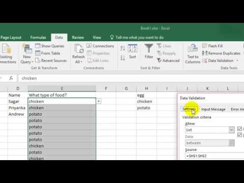
Dependent drop-down lists where you choose a country and magically the next drop-down list only displays the states for that country used to be laborious to set up and maintain, but now that we have dynamic array formulas, we can make them dynamic, so they automatically grow with your data.
In this video, I’m going to show you two approaches, one that’s relatively straight forward but has some limitations, and one that overcomes those limitations using a trick that is mind blowing.
CORRECTION: I learned this technique from Ceasr of the @Excelambda channel. Check out his work.
LEARN MORE
===========
⏲ TIMESTAMPS
==============
0:00 Method №1
5:14 Method №2
#Excel #ExcelTricks #ExcelDataValidation
 0:11:15
NEW Excel Drop-Down Lists That Adapt to Your Data
 0:01:01
How to create a drop-down list in Microsoft Excel
 0:05:20
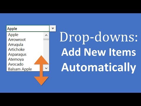
Add New Items To Excel Drop-down Lists Automatically In Seconds!
 0:08:37
Excel Drop Down List Tutorial
 0:02:01
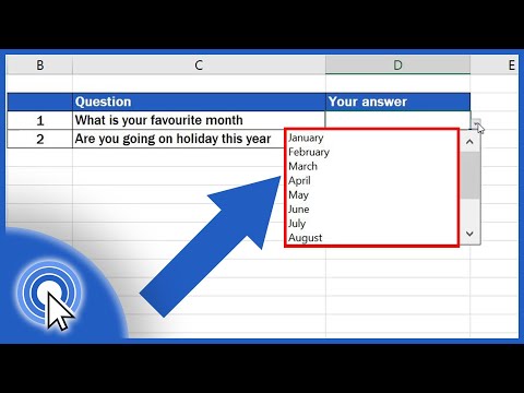
Unique Drop Down Lists that Automatically Update with New Values
 0:01:22
How to create drop down list in excel with multiple selections
 0:05:31
Excel Drop Down List Including Cell Colour Change
 0:03:22
How to Create a Drop-Down List in Excel
 0:10:02
Dynamic Excel Drop Down Lists - PLUS how to get SEARCHABLE Drop Down Lists!
 0:03:50
Excel Create Dependent Drop Down List Tutorial
 0:01:32
How to add a drop-down list in Microsoft Excel
 0:07:16
Create multiple dependent drop-down lists in Excel [EASY]
 0:13:08
Advanced Excel - Data Validation and Drop-Down Lists
 0:15:42
Create SMART Drop Down Lists in Excel (with Data Validation)
 0:09:36
How to use XLOOKUP to Create Dependent Drop-Down Lists in Microsoft Excel
 0:08:04
Auto-Populate Other Cells When Selecting Values in Excel Drop-Down List | VLOOKUP to Auto-Populate
 0:04:44
Add New Items to Excel Drop Down List
 0:09:17
Crazy Drop Down Lists for Excel
 0:01:36
How to edit drop down list in Microsoft excel
 0:00:27
Create a drop down list in Google Sheets
 0:11:57
Create Multiple Dependent Drop-Down Lists in Excel (on Every Row)
 0:09:48
How to Create Multiple Dependent Drop-Down Lists in Excel | Automatically Update with New Values
 0:06:09
How to Create Searchable Drop Down Lists in Excel with ZERO Effort!
 0:11:10
Dependent Drop Down List in Excel Tutorial
Комментарии