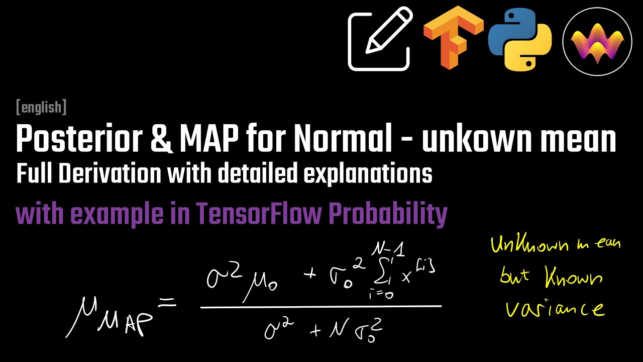
Posterior for Gaussian Distribution with unknown Mean

Corrupt or Noisy datasets are ubiquitous in Machine Learning. Hence, the right approach is to always work with regularization. However, if we want to infer the mean of a dataset by the MLE (which leads to the classical known average) we are highly unregularized and spurious effects in the dataset can greatly affect our estimate.

How can we encode prior knowledge in order to find a more robust estimate? This can be done by putting a prior on the mean of the Normal while keeping the standard deviation/variance fixed. In this video we will derive the posterior and the Maximum A Posterior Estimate step-by-step.

After the derivation we will look at an example in TensorFlow Probability where we compare MLE and MAP for perfect and corrupt data.

-------

-------

Timestamps:
00:00 Introduction
00:56 The Directed Graphical Model
02:22 The Likelihood
04:20 What is the prior for mu?
05:20 The Hyper-Parameters
06:20 Defining Distributions
06:45 The joint distribution
10:06 Bayes Rule
11:11 Proportionals to get the Posterior
11:37 Deriving the Posterior
19:05 Completing the Square
21:14 Deriving the Posterior (cont.)
23:22 Discovering the Posterior Normal
25:30 Mean of the Posterior Normal
25:55 Discussing the Posterior Mean
27:33 Std of the Posterior Normal
27:50 Discussing the Posterior Std
28:57 Maximum A Posterior Estimate
30:17 TFP: Creating a dataset
31:17 TFP: Computing the MLE
31:32 TFP: Defining prior knowledge
32:17 TFP: Computing the MAP
33:11 TFP: Comparing MLE and MAP
33:33 TFP: Creating the Posterior Distribution
33:51 TFP: MLE vs MAP for corrupt data
37:00 Outro

[orjihvy]

The TensorFlow Probability example was really helpful again. I was wondering though, if there is any intuition as to why sigma_N is substantially smaller than sigma_true and sigma_0.