Excel Multi Color Data Bars using Conditional Formatting

Learn: The Quick & easy way on Excel Multi Color Data Bars using Conditional Formatting

In this video, you will learn:
1. Excel Multi Color Data Bars using Conditional Formatting
2. Excel data bars

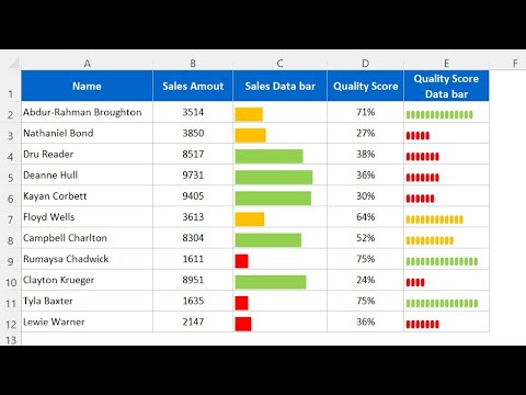
Excel Multi Color Data Bars are the combination of Data and Bar Chart inside the cell, which shows the percentage of selected data or where the selected value rests on the bars inside the cell. The data bar can be accessed from the Home menu ribbon’s Conditional formatting option drop-down list. If we go there, we will be able to see Gradient Fill and Solid Fill Data bar. Whereas gradient fill uses the shades in the cell with values, and solid fill uses the solid dark color fill. Suppose we have a list of 15 numbers, and if we use Data Bars, then it will automatically calculate the length of the bars it should keep for all the selected values inside the cell.
How to Add Data Bars in Excel?

Firstly, let’s consider the difference between a chart and a data bar. For this, I have taken some product data from products A to K to show the numbers in graphics.
For this data, let me apply a simple Column Bar Chart for Dept. A.
Step 1: Highlight the Entire data table in Dept. A column, then Go to Insert and click on a Column chart. Choose the second option there.
Step 2: Now, we have a simple Column chart for our data.
Wow!! This looks good to go and present. But wait, we have more interesting graphics which show the bars inside the respective cell itself; I am sure you will be amused at seeing them.
We will add excel Data bars for this data which show the bars inside the cell along with the numbers. Follow the below steps to add data bars in Excel.
Step 3: Select the number range from B2 to B12.
Step 4: Go to the HOME tab. Select Conditional Formatting and then select Data Bars. Here we have two different categories to highlight; select the first one.
Step 5: Now, we have a beautiful bar inside the cells.
The highest value has the largest bar in this group; the least value has the short bar. This is automatically picked by excels conditional formatting only.
In other words, In case if you do not want to see numbers in the cell, but want to see only bars in the cell, you can choose to show only bars instead of showing both of them. In order to show only bars, you can follow the below steps.
Step 1: Select the number range from C2:B12
Step 2: Go to Conditional Formatting and click on Manage Rules.
Step 3: Click on New Rule.
Step 4: A new dialogue box pops up, go to the Format Style section, select Data Bar from the drop-down list and checkmark ‘’Show Bars Only” and then click OK.
Step 5: Now, we will see only bars instead of both numbers and bars.
However, Excel Data bars work for negative numbers as well. I have a student’s three-semester competitive exam scores. Due to negative marking, some of the students in some of the exams got negative marks.
By looking at the data, suddenly you cannot tell which student got negative marks in exams. We need some highlights here also to identify the top scores in each exam very quickly. This can be done by using the Data Bar technique in conditional formatting. To get this result:
First Step 1: Select the Semester 1 Scores range of cells from F2:F12
Step 2: Go to Conditional Formatting and select Data bars. Select gradient fills but does not select red bars because we have negative numbers here. All the negative numbers will be represented by red bars. You can choose either the first option or the second option without the red bar.
Step 3: Now we have bars. We can quickly identify the negative scores easily.
Step 4: For other remaining 2 semesters, you don’t apply conditional formatting one by one; rather, you can copy the currently applied conditional formatting range and paste it as formats.
Copy the current conditional formatting range by pressing Ctrl + C.
Step 5: Select the remaining 2 semesters range. Press ALT + E + S + T. This is the shortcut key for pasting the only format of the copied cells.
Step 6: We will have conditional formatting data bars for all the exams now.
Always note that:
• There are two kinds of Data Bars available in Excel. Select Gradient if you present both bar and numbers together or if you are showing only bars select Solid.
• You can change the color of the bar under the Manage Rule and change the color there.
• When the data includes negative values, bars will be created from half of the cell, not from the left-hand side of the cell.

……………………………………………………………………………………………………………………….

For more simple and easy to follow How to videos,

Click the Link Below to subscribe:

Join this channel to get access to the perks:

#exceldata #bars #formatting

LearnexcelwithT

[cnncnn]

You are an excellent teacher. Thank you

[RevoZtuns]

Is there a way to apply 3 colour scale gradient to a data bar? e.g. Green - Amber - Red --> all within a single data bar based on Min and Max value (e.g. 1-5)?