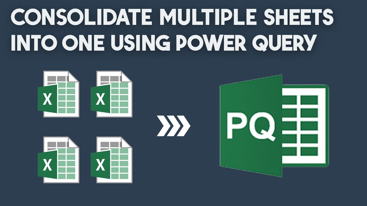
Combine Multiple Worksheets into one using Power Query

Combine Multiple Worksheets into one using Power Query [Consolidate Data in Excel]

Today, I'm gonna show you how to combine multiple Worksheets into one using Power Query. Each tab contains more than 100,000 records.
Click the Data tab. Choose 'Get Data From Excel Workbook'.Browse and import the Excel file. In the Navigator pane, you can see the Workbook and all Worksheets. Click the folder icon. Then click the Transform Data button. The Power Query window will appear. We only need to keep the Data column that contains tables. Click the column header to select the entire column. Locate the Manage Column Group. Use the 'Remove other columns' command. Click the expand icon. Make sure that the name prefix box is unchecked. Click OK to get back to the Power Query window. We are consolidating multiple sheets, so there are multiple headers. It is worth to hide these rows to keep our data clean. Select Column 4 and uncheck the records that contain the Items keyword. In the first column, we have dates, so it is worth changing the default number format to date. Change the column names. Using this step, our output will be easy to read. Click the close and load button. Power Query will load and merge all Worksheets into a single Worksheet.

Chapters:

0:00 Intro
0:11 Consolidate Multiple Worksheets into one using Power Query
0:18 Import Data
0:35 The Power Query window
0:38 Remove unnecessary columns
1:06 Filter duplicated headers
1:26 Merge Worksheets into one

#msexcel #excel #exceltips #exceltricks #excelformula #productivity #datacleaning #datacleansing #powerquery #powerquerytutorial

[muhammadsaeedakhtar]

For my future reference, this was the one that works!!! loved

[Harpreet]

For my future reference, this was the one that works!!!

[J-yniw]

Great video. What if I wanted changes made to items in the final, merged list, to reflect back to their source tables/files?

[MVls-su]

Thank you so much. Is there a way to combine multiple workbooks into one workbook, but each workbook would be saved in a separate sheet? I need multiple workbooks combined because they will go to the same person, but each workbook needs to be it's own sheet. I appreciate any help anyone can give me!

[metiel]

thanks! step by step was helpful. however after merging data and the final rows exceed the Excel limited of 1M rows, is there a solution for this?

[Non-disjunction]

So how to do this if the tables use the variable 'projects' as the key value, but have different columns?

[isasadikhov]

Thanks for the video, what if it worksheets are not in table format?

[larrybud]

Any way to combine the tabs into the same workbook? Couldn't figure out how I can do this within a single file.

[djphilter]

How do you combine multiple Queries, the section on the left of the Power Query Editor, into one and or how do you combine multiple worksheets that each query makes when I click on close and load; all into one worksheet?

[sethvanesschoten]

Jesus Christ, hire a voice over artist.