Regression Assumptions Explained in Detail Part 1 | Econometrics Lecture

In previous videos, we have discussed what regression is and how to interpret the regression coefficients. in this video we are going to understand what are the assumptions that must be fullfiled before we can use OLS regression.
So let's get started. On the screen you would see our basic regression model. Whether wage is our dependent variable and it is fuction of education and experience of an individual and plus an error term.
If we run this equation using some real life data, we will get these numbers. Now in this video I am assuming that you are already familiar with the interpretation of these number, If not then I suggest you watch my previous videos.
Now we can only rely on these number if the assumptions that we are going to discuss in this video holds. If the regression assumptions do not hold, then these numbers are misleading and interpreting them will lead to a wrong conclusion..
So lets explore these assumptions. Let me first list down these assumptions then we explore each of them in detail.
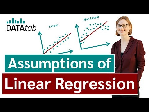
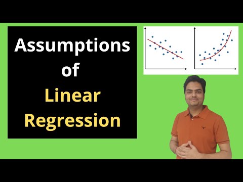
The first assumption is linearity : it says that the model should be linear in parameters
Then we have the homoscedasticity assumptions which states that the variance of error term should be constant
The no multicollinearity assumptions: it states that explanatory variables should not be correlated with each other
No autocorrelation : that is the error terms should not correlated with other error terms, and this assumptionsis mostly important in time series data
Normality assumtions: This assumption states that the error term should be normally distributed i.e. is to say that error term should have a bell shape distribution
Non-constatnt X : No most of the books will take this assumption as obvious and will not state it. But iin this video we are going to explicity state it. This assumpitons says that variables should vary. That is they must not be constant
Again this assumption is also normally not stated. The assumptions states that number of observations should be greater than number or explanatory variable or parameter in the equation
Exogeneity. The assumption demands that explanatory or the independent variable should not be correlated with error term.
And lastly, The regression equation should have a correct fuctional form.

Lets dive deeper into the linearity assumption

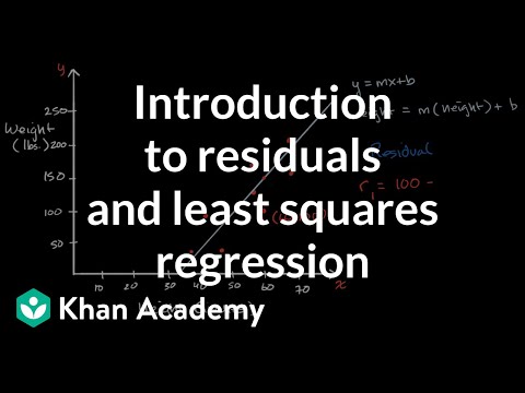
So here we have our y-axis
And the x-axis
On y-axis we have our dependent or the outcome variable , which in this case in wage
On x-axis we have our independent or the predictor variable which in this case in education. Now for the sake of simiplicity we are just assuming one predictor variable but the same idea can be extendend to more than one predictor.
We have a bunch of observations which we have collected
So lets call them observed values
Aaaaaaand we have our fitted line
Now this line represents that there is a linear relationship between education and wage, and by linear we mean a relationship that is represented by a straight line.
Now when we talk about linearity, it would be more fruitfull if we divide it into two parts
So a model can be linear in variables
Or it can be linear in parameter. Linearity in variable means that the variable must have a power of 1 only i.e it do not have any exponent, nither square root or the variable is not multiplied or divided by any other variable

Best 10 Introductory Econometrics Books

Data Management Using Stata: A Practical Handbook by Michael N. Mitchell

A Gentle Introduction to Stata, by Alan C. Acock

A Visual Guide to Stata Graphics, by Michael N. Mitchell

Regression Models for Categorical Dependent Variables Using Stata, by J. Scott Long and Jeremy Freese

Disclaimer: Some links are affiliate links that help the channel at no cost to you.

[lotus]

Awesome Video! Well explained! Quick question..

How could you manipulate the design of an experiment to reduce teh amount of error resulting in data?