How to Use HLookup Function In Excel

How to use HLOOKUP Function in Excel

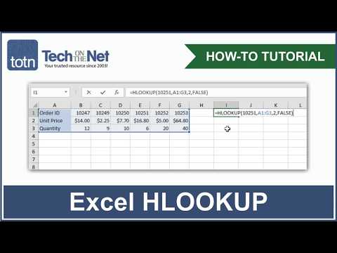
HLOOKUP Function in Excel stands for “Horizontal Lookup.” This function searches for a specific value in a row to return a value from a different row from the same column.

The HLOOKUP function looks like this:
=Hlookup(lookup_value, table_array, row_index, [range_lookup] )

An HLOOKUP function has four parameters:

Lookup value: The value you need to lookup.

Table Array: The range from where you want to find your value. It could be a table also. Remember your lookup value must be in the first row. So, start the range by keeping the value you want to find in the first row.

Row index: This is the row number from which you want to retrieve data.

Range lookup: this is an optional argument. You need to confirm if you want an exact match or approximate match. The Default here is TRUE, which indicates an approximate match. If you need an exact match, then select FALSE.

#Hlookup #Function #Excel

Thanks for watching.
----------------------------------------------------------------------------------------
Support the channel with as low as $5
----------------------------------------------------------------------------------------
Please subscribe to #excel10tutorial

Here goes the most recent video of the channel:

Playlists:

Social media:

[robertnegron]

I can barely understand a word you are saying...Your accent is killing me!