How to Create lookup tables in Excel

Показать описание

Learn how to use the vlookup formula in Excel. Create a logical function and send it to find a logical value. In this manner, you can have your lookup table.

Vlookup in Excel is considered kind of tricky by most users. We will teach you how to apply vlookup. In the formula, you have to provide the cell where the results would be displayed, the data range, the column you are referencing it to and whether the condition is true or false. It is a logical function and helps people in real life situations when they are trying to maintain a car database or parts database.
In this tutorial, we will show you how to create a lookup table in Excel.

Step # 1 -- Name your data range
When you are working with large amounts of data and want to find a specific row, you can use the lookup function.
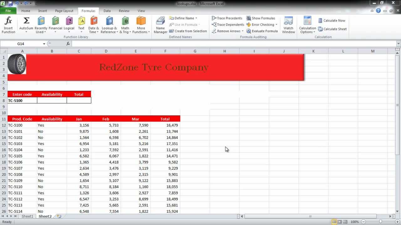
First of all, give your data a name. Click anywhere on the data and press "ctrl + a". Now go to the name bar and give it a name. In this tutorial, we have named it "Data".

Step # 2 -- Insert Vlookup
In the video, we will start typing the function in cell "b8".
Write =vlookup(a8, data, 2, false)
Now let us explain the vlooklup in Excel. In the tutorial, we have written A8 because that's the code by which we will look up the data. "data" has been entered in the function because that is the name of our data range. Two is inserted for the second column "availability". "false" is entered in the function at the very end because we want to find the exact match. If "true" was entered then it would have searched for a close match.

Step #3 -- Modify the Vlookup formula
Similarly for total the same function was used. However instead of writing "2" in the function, we have written "6" because "total" is in the sixth column.
Now whenever we change the value of cell "a8" in the tutorial, the results of "availability" and "total" are re-worked accordingly.

Рекомендации по теме

Комментарии

❗ Subscribe To Our Main YouTube Channel

howtechoffice

For beginners, what the video doesn't do is tell you how the table got there from the start. A table is not just a spreadsheet with headers. You have to insert a table first from the Insert tab. You do this by clicking anywhere in the rows and columns of your "table" array and type Ctrl-A to automatically select the rows and columns of the array. Then on the Insert Tab, click the "Table" icon. A "Create Table" dialog box pops up with its given dimensions. Click OK and it will be given a default name such as "Table1". Finally, the hidden Table Tools Design tab will magically appear showing you the assigned name in the Table Name field on the far left. Then the video begins from that point.

jimlemay