filmov
tv
How to Freeze Top 3 Rows in Excel
Показать описание
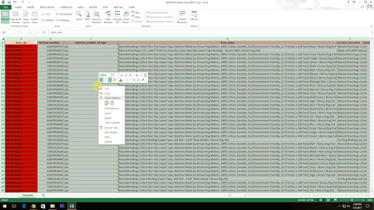
Instructions on how to freeze the top 3 rows on Excel:
Step 1: Highlight the first two rows. Right click on it and hide it.
Step 2. Under Menu go to View, Freeze Panes, then select Freeze Top Row.
Step 3. Now, unhide the first two rows. And there you have it.
Step 1: Highlight the first two rows. Right click on it and hide it.
Step 2. Under Menu go to View, Freeze Panes, then select Freeze Top Row.
Step 3. Now, unhide the first two rows. And there you have it.
 0:00:48
How to Freeze Top 3 Rows in Excel
 0:00:34
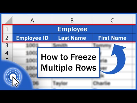
How to Freeze More Than One Row in Excel
 0:02:01
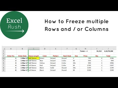
How to Freeze Multiple Rows and or Columns in Excel using Freeze Panes
 0:00:43
Excel Freeze Top Row and First Column (2020) - 1 MINUTE
 0:02:45
How to Freeze Multiple Rows in Excel (Quick and Easy)
 0:02:16
How to Freeze Multiple Rows and Columns in Excel
 0:03:35
HOW TO FREEZE MULTIPLE ROWS AND COLUMNS (EASY 2-STEP METHOD)
 0:03:36
How to Freeze Panes in Excel
 0:09:32
Bgmi Episode 7 - Godlike qualified for semifinals । After three years of struggle Godlike qualified...
 0:02:02
How to freeze rows and columns at the same time in excel 2019
 0:02:36
How to Freeze Multiple Rows and Columns in Excel Using Freeze Panes (Lock Rows and Columns in Excel)
 0:01:26
How to Freeze Multiple Rows and or Columns in Google Sheets using Freeze Panes
 0:04:33
How to Freeze Multiple Columns and Rows in Microsoft Excel 🔥
 0:03:01
How to Freeze Top Row and First Column in Excel (Quick and Easy)
 0:01:18
How to Freeze a Row in Excel [ MAC ]
 0:02:53
How to Freeze Selected Rows In Excel?
 0:05:05
How to Freeze Multiple Rows and or Columns in Excel using Freeze Panes in Malayalam
 0:03:32
How to ACTUALLY freeze and why I dislike Proguides/Skillcapped
 0:04:47
How to Freeze Multiple Rows and Columns in Excel | Freeze Rows and Columns in Excel
 0:06:22
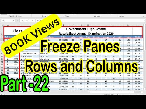
How to Freeze Multiple Rows and Columns in Excel using Freeze Panes Part 22
 0:00:29
How to *FREEZE* or Pause Video on CapCut!
 0:01:13
How to Freeze Rows & Columns in Numbers
 0:01:51
Google Sheets: How to Freeze Rows and Columns | Freeze Top Row | Freeze First Column
 0:01:06
How to Freeze Header Rows and Columns in an Apple Numbers Spreadsheet
Комментарии