filmov
tv
R Stats: Multiple Regression - Variable Preparation

Показать описание
This video gives a quick overview of constructing a multiple regression model using R to estimate vehicles price based on their characteristics. The video focuses on how to prepare variables while employing a stepwise regression with backward elimination of variables. The lesson explains how to transform highly skewed variables (using Log10 transform) and later report their characteristics, how to check variable normality and their multiple collinearity (using Variance Inflation Factors) and their extreme values (using Cook's distance). The process will be guided by the measures of model quality, such as R-Squared and Adjusted R-Squared statistics, and variables' p-values, which represent the level of coefficient confidence. As always, the final model will be evaluated by calculating the correlation between the predicted and actual vehicle price for both the training and validation data sets, with correction for the previously transformed variables. The explanation will be quite informal and will avoid the more complex statistical concepts. Note that visual presentation and interpretation of multiple regression results will be explained in the next lesson.
The data for this lesson can be obtained from the well-known UCI Machine Learning archives:
The R source code for this video can be found here (some small discrepancies are possible):
The data for this lesson can be obtained from the well-known UCI Machine Learning archives:
The R source code for this video can be found here (some small discrepancies are possible):
 0:07:43
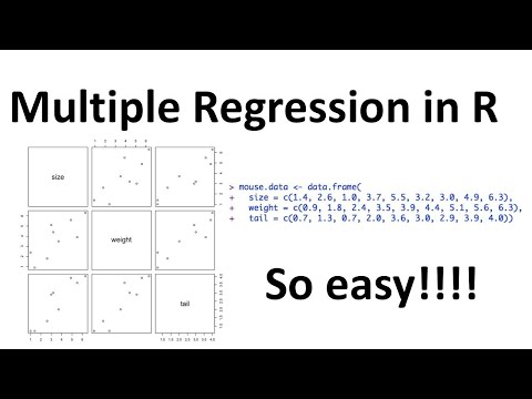
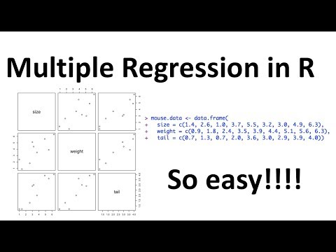
Multiple Regression in R, Step by Step!!!
 0:05:19
Multiple Linear Regression in R | R Tutorial 5.3 | MarinStatsLectures
 0:07:43
Multiple Regression in R, Step-by-Step!!!
 0:10:46
Multiple regression: how to select variables for your model
 0:05:25
Multiple Regression, Clearly Explained!!!
 0:09:26
Multiple regression in R: example
 0:04:05
Multiple Regression | ANOVA Table | F-Test | R-square | Standard Error
 0:20:48
Multivariable Linear Regression in R: Everything You Need to Know!
 1:14:06
Class 11: Generalized Measurement Models (Lecture 04a, part 1, Bayesian Psychometric Models, F2024)
 0:09:57
Quick tutorial on how to run Multiple regression in R
 0:13:12
Multiple linear regression in R
 0:08:11
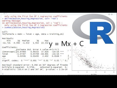
How To... Make a Prediction using a Multiple Linear Regression Model in R #102
 0:09:48
Multiple linear regression with interaction in R
 0:05:25
Multiple Regression, Clearly Explained!!!
 0:11:01
How To... Create a Multiple Linear Regression Model in R #101
 0:05:01
Linear Regression in R, Step by Step
 0:33:49
Multiple linear regression using R studio (Aug 2022)
 0:08:06
Multiple Regression | Coefficients – Interpretation, C.I, Hypothesis Testing
 0:22:05
R Stats: Multiple Regression - Variable Preparation
 0:12:47
Multiple regression. How to deal with Outliers and Colliniarity
 0:25:28
Multiple Linear Regression using R ( All about it )
 0:28:40
Adding variables to your multiple regression model
 0:06:02
Multiple Linear Regression with R | 3. Model
 0:22:13
R Stats: Multiple Regression - Data Visualisation
Комментарии