filmov
tv
Second order differential equation for spring-mass systems

Показать описание
Let's look at modeling the motion of a spring-mass system (a harmonic oscillator) using a second-order differential equation. From Newton's Second Law, we arrive at mx'' + cx' + kx = 0 (or a forcing function), where x(t) is the position of the spring-mass over time, m is the mass, c is the damping coefficient, and k is the constant from Hooke's Law. We focus on the effects of damping and how to detect what kind of damping a spring-mass system has based on the roots of the characteristic equation.
Four types of spring motion are discussed based on the roots: undamped (no damping force), underdamped (small damping), critically damped (damping force just prevents oscillation), and overdamped (large damping). Different damping leads to different behaviors, which we can illustrate with MATLAB simulations.
#mathematics #math #differentialequations #ordinarydifferentialequations #stemeducation #harmonicoscillator #hookeslaw #physics #matlab #matlabsimulation #iitjammathematics
 0:25:17
Second Order Linear Differential Equations
 0:41:28
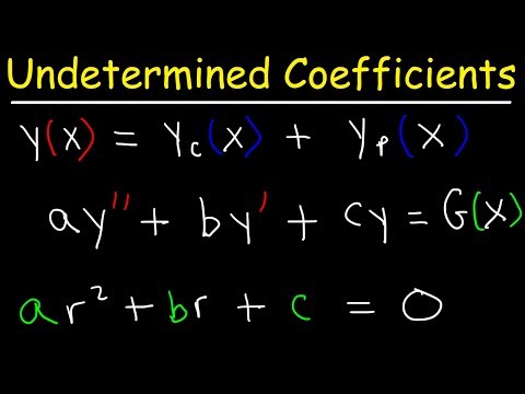
Method of Undetermined Coefficients - Nonhomogeneous 2nd Order Differential Equations
 0:06:41
How to Solve Constant Coefficient Homogeneous Differential Equations
 0:11:19
The Theory of 2nd Order ODEs // Existence & Uniqueness, Superposition, & Linear Independence
 0:32:54
Solving Second Order Differential Equations
 1:19:11
4. Second-Order Equations
 0:12:44
Undetermined Coefficients: Solving non-homogeneous ODEs
 0:11:44
Second order homogeneous linear differential equations with constant coefficients
 2:03:18
Lec-03 | Homogeneous & Exact Differential Equation | Differential Equation | Engineering Mathema...
 0:37:02
Second-Order Ordinary Differential Equations: Solving the Harmonic Oscillator Four Ways
 0:19:20
Second Order Equations
 0:04:35
Homogeneous Second Order Linear Differential Equations
 0:10:21
2nd Order Linear Differential Equations : P.I. = trig type : ExamSolutions
 0:03:02
How To Solve Second Order Linear Homogeneous Differential Equation
 0:47:14
Reducible Second Order Differential Equations, Missing Y (Differential Equations 26)
 0:27:16
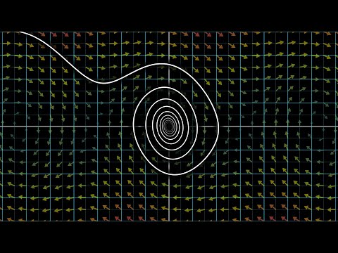
Differential equations, a tourist's guide | DE1
 0:26:58
Nonhomogeneous 2nd-order differential equations
 0:41:00
How to solve second order differential equations
 0:25:18
Solving Non-Homogenous Second Order Differential Equations
 0:26:57
🔵18 - Second Order Linear Homogeneous Differential Equations with Constants coefficients
 0:14:29
Reduction of orders, 2nd order differential equations with variable coefficients
 0:09:27
Second order differential equations with variable coefficient
 0:11:58
Introduction To Second Order Linear Homogeneous Differential Equation
 0:31:31
More Examples of Second Order Differential Equations
Комментарии