filmov
tv
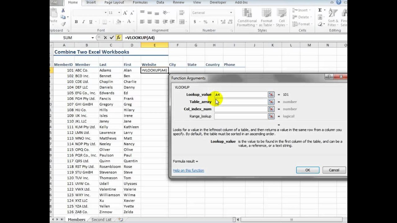
How to Combine 2 Excel Workbooks Using VLOOKUP
Показать описание
This is a request from one of my viewers. In his organization, two people were working on this project and he needed to produce a consolidated Excel worksheet.
Fortunately, when I look at the workbooks he sent me, I noticed that both had a MemberID field that contained the Unique Account Numbers. With this knowledge, I decided that the VLOOKUP Function would be the easiest way to complete this task.
Here is a list of the Excel Techniques that I demonstrate in this tutorial:
* Move or Copy a worksheet to another Excel Workbook
* Create a Named Range to use as the "Table_array" in the VLOOKUP Function
* Use "Mixed Cell References" - e.g. $A4 - in VLOOKUP Function
* Use FALSE as the optional 4th Argument in VLOOKUP to produce an "Exact Match"
* Use IFERROR Function to prevent Error Messages from appearing
Danny Rocks
The Company Rocks
 0:01:35
How Do I Merge Two Excel Spreadsheets
 0:05:58
COMBINE Multiple Excel WORKBOOKS into One | ExcelJunction.com
 0:03:08
Merge Multiple Excel Files into 1 File in just few Seconds !!
 0:09:05
Excel - Merge Data from Multiple Sheets Based on Key Column
 0:08:22
How to Combine 2 Excel Workbooks Using VLOOKUP
 0:02:11
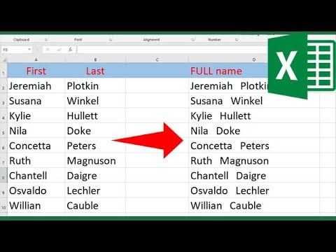
How to merge two columns in Excel without losing data
 0:04:52
How to link two files in Excel - 2 ways to solve the problem
 0:07:27
AWESOME Excel trick to combine data from multiple sheets
 0:05:54
Fix Excel Dates with This Simple Trick using DATE function
 0:10:29
Easiest way to COMBINE Multiple Excel Files into ONE (Append data from Folder)
 0:02:09
How to Combine Multiple Excel Workbooks into one Workbook | Excel Tutorials for Beginners
 0:09:04
How to Merge Excel Files (Without Using VBA) - 4 Easy Ways
 0:06:02
How to Join Tables using VLOOKUP formula in Excel
 0:08:25
How to connect two tables in Excel - With Example Workbook
 0:00:45
Merge OR Concatenate two columns in Ms Excel
 0:01:22
Excel Tips and Tricks #36 How to combine two graphs into one
 0:05:50
Excel Workbook Fusion: Combine Workbooks with Common Column - Episode 2216
 0:06:29
Combine Data from Multiple Sheets into One Sheet In Excel | Consolidate Tables into a Single Sheet
 0:02:17
How To Combine Two Columns In Excel
 0:11:47
EASY Trick to COMBINE Multiple Excel files into ONE with Power Query
 0:01:52
How Do You Merge Two Excel Files And Remove Duplicates
 0:06:07
Combining Data From Multiple Cells in Excel
 0:00:50
How to combine two cells in excel
 0:06:56
Excel Magic Trick 1412: Power Query to Merge Two Tables Into One Table for PivotTable Report
Комментарии