filmov
tv
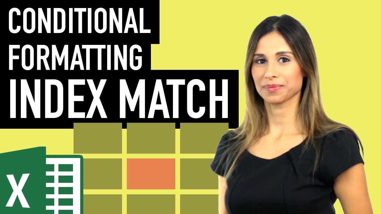
How to Conditional Formatting the Lookup Result in Excel Data Table (Index Match)

Показать описание
Find out how you can highlight values inside your data set based on a condition. In this example, we are going to conditionally format the result of our lookup formula (I use INDEX Match here) to conditionally format that same value that we find inside the original data set.
The tricky part is to get the conditional formatting formula correct. Just remember, one reason why your conditional formatting formulas might not work can be due to the wrong usage of the dollar sign for fixing the cell references (i.e. absolute, versus relative referencing - and sometimes you need a mix of the two).
Links to related videos:
🚩Let’s connect on social:
Note: This description contains affiliate links, which means at no additional cost to you, we will receive a small commission if you make a purchase using the links. This helps support the channel and allows us to continue to make videos like this. Thank you for your support!
#excel
Conditional Formatting in Excel Tutorial
Excel Conditional Formatting with Formula | Highlight Rows based on a cell value
Master Conditional Formatting in Excel (The CORRECT Way)
How to: Use Conditional Formatting Rules in Sheets
Conditional Formatting Formulas - Mystery Solved with 3 Simple Rules
MS Excel - Advanced Conditional Formatting
Excel: Conditional Formatting
Conditional Formatting in Excel | Excel Tutorials for Beginners
Excel Conditional Formatting in Depth
Advanced Conditional Formatting in Excel | Conditional Formatting in Excel
Excel How To: Format Cells Based on Another Cell Value with Conditional Formatting
Excel Essentials -- Level UP! -- Conditional Formatting for Due Dates and Expiration Dates
5 Conditional Formatting tips to make you a rock star at work 🤘
MS Excel - Conditional Formatting Part 1
How to Conditional Formatting the Lookup Result in Excel Data Table (Index Match)
Apply Conditional Formatting to an Entire Row - Excel Tutorial
Excel Conditional Formatting using Formulas
Excel Conditional Formatting Advanced Technique
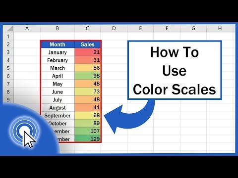
How to Use Color Scales in Excel (Conditional Formatting)
Excel Conditional Formatting based on Another Cell | Highlight Cells
Conditional Formatting in Excel | Highlight Marks Pass/Fail #shorts #excel
Four SMART Ways to use Custom Formatting instead of Conditional Formatting in Excel - Part 1
Conditional Formatting Based on Another Cells Values – Google Sheets
MS Excel - Conditional Formatting Part 2
Комментарии
 0:06:43
 0:09:40
 0:10:37
 0:00:27
 0:04:25
 0:05:20
 0:03:46
 0:20:59
 0:17:39
 0:05:02
 0:09:29
 0:06:54
 0:12:00
 0:10:42
 0:09:25
 0:04:21
 0:09:23
 0:05:51
 0:03:42
 0:01:30
 0:00:29
 0:16:12
 0:03:34
 0:05:55