Scalar line integrals, Multivariable Calculus

We derive expressions for the scalar line integral of f over a curve C in its domain. Three examples of computing scalar line integrals. (This is Multivariable Calculus Unit 6 Lecture 5.)

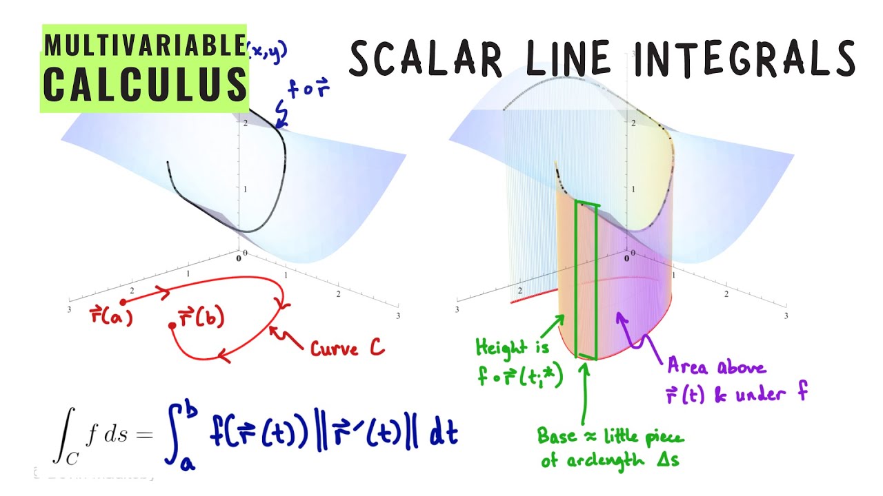
Consider the graph of 𝑧=𝑓(𝑥,𝑦) as a surface in ℝ3. This function may be defined over the entire 𝑥𝑦-plane. However, with line integrals we restrict our attention to a curve in the domain and the values the function takes along it.

Visually, we examine a curve segment 𝐶 residing in the 𝑥𝑦-plane and parametrized by 𝐫(𝑡) with 𝑡 from 𝑎 to 𝑏. The graph of 𝑓 just over 𝐶 forms a "curtain" in space. We aim to determine the area of this curtain shape.

(The derivation is done for a function of two variables over a curve in a plane, but the concept generalizes to functions of three variables evaluated along a space curve.)

We approximate this area through an assembly of rectangles, where each rectangle's height is the function value at points along 𝐫(𝑡), and the base is a segment of approximated arc length Δ𝑠.

The curtain area approximation translates into adding up the areas of these rectangles, leading to the scalar line integral expressed as ∫_𝐶 𝑓 𝑑𝑠.

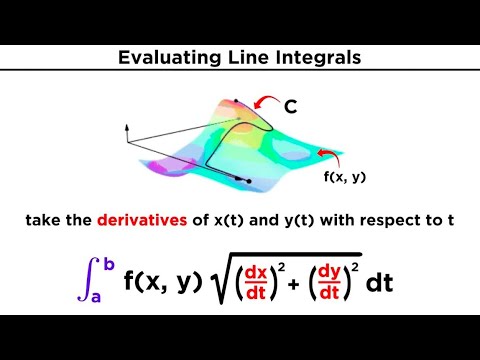
In practice, we utilize the relationship between arc length and speed, 𝑑𝑠/𝑑𝑡=‖𝐫′(𝑡)‖. This transformation results in the commonly used computational formula for scalar line integrals:

∫_𝑏^𝑎 𝑓(𝐫(𝑡))‖𝐫′(𝑡)‖ 𝑑𝑡.

#calculus #multivariablecalculus #mathematics #lineintegral #iitjammathematics #calculus3 #vectorcalculus

[eswyatt]

This is amazing. Same stuff I've seen and done 100 times, but new ways of looking at it!

[kofhk]

Could you explain why 08:57 f(r(t)) = 8t?