How to Create a Pivot Table in MS Excel | How to Organize and Analyze Data in MS Excel

In this video, we’ll be showing you how to create a basic pivot table in Excel.

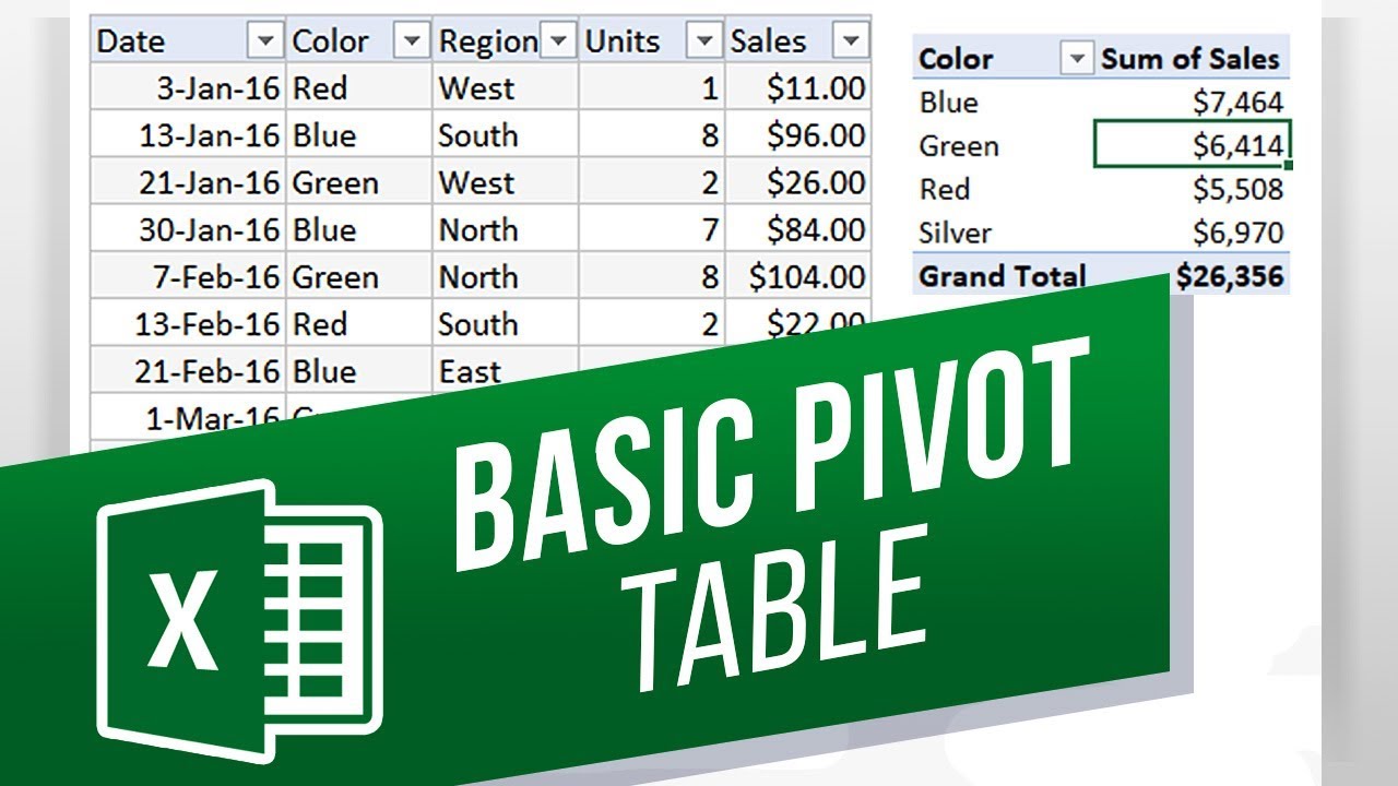
PivotTables can reorder the structure of a set of data like this. They’re commonly used for extracting and calculating the important information and moving it to a separate table. Let’s say you have a huge data table, but you only need a small section. PivotTables are the way to go.

We will create a PivotTable that isolates certain data from a large table.
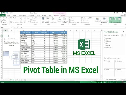
➡️ Select data and create a PivotTable from the Insert tab.
➡️ Check the relevant boxes for categories of data you want.
➡️ Explain the four controls of PivotTables (Filters, Columns, Rows, Values).
a. The top item in the Rows will be the main categories in the PivotTable.
b. Any items after the first in Rows will be sub-categories.
c. The same is true for Columns. (show difference between Rows and Columns by dragging items to each)
d. Values can be changed to be sums, counts, and other options to show the total amount of money a seller has made.
e. If a filter is added, such as a Date item, the entire PivotTable can be filtered by the user to a specific date.

PivotTables are great for reordering and summarizing data in large tables.

❓💬 What other methods do you use to organize your data? Please let us know in the comments.

#HowTech #Excel
--------------------------------------------------------------------------------------------------------------