filmov
tv
Excel Conditional Formatting with Charts - Two Examples

Показать описание
Apply Conditional Formatting to your Excel charts to visualise the metrics that you need to see.
Excel does not have a Conditional Formatting feature that can be applied to charts. However, there is a simple way that we can do this.
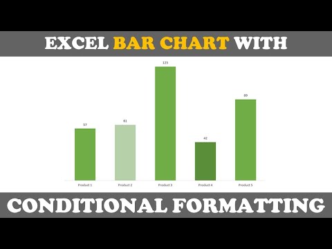
You first need to write a logical formula to identify and show the values you want and hide the ones you don't. The IF function is perfect for this.
We then create our chart from this data and overlap the data series giving the appearance of Excel Conditional Formatting with charts.
You can apply any criteria that you want. Great for visualising actuals against target values, or the max and min values of a chart.
Find more great free tutorials at;
*** Online Excel Courses ***
Connect with us!
Excel does not have a Conditional Formatting feature that can be applied to charts. However, there is a simple way that we can do this.
You first need to write a logical formula to identify and show the values you want and hide the ones you don't. The IF function is perfect for this.
We then create our chart from this data and overlap the data series giving the appearance of Excel Conditional Formatting with charts.
You can apply any criteria that you want. Great for visualising actuals against target values, or the max and min values of a chart.
Find more great free tutorials at;
*** Online Excel Courses ***
Connect with us!
 0:01:31
How to Make a Graph Change Color Based on Value | Conditionally Formatting Charts
 0:10:23
Simple Excel Trick to Conditionally Format Your Bar Charts
 0:05:23
Conditional formatting for Excel column charts
 0:09:25
Apply Conditional Formatting to Microsoft Excel Charts
Excel Conditional Formatting with Charts - Two Examples
 0:09:49
How to use Conditional formatting in Excel Chart
 0:03:49
How to Apply Conditional Formatting Rules to Your Excel Column Charts
 0:12:05
How to Apply Conditional Formatting in Excel Charts
 0:00:50
Do You Know How To Activate Automatic Data Entry Form In Excel?|#excel#interviewquestions#dataentry
 0:01:36
How to Create Bar Charts Using Excel Conditional Formatting
 0:11:32
Conditional Formatting in Charts?!
 0:10:37
Master Conditional Formatting in Excel (The CORRECT Way)
 0:11:52
Conditional Formatting for Graphs and Charts in Excel
 0:06:55
Excel Bar Chart - Conditional Formatting | FREE Download
 0:03:47
Conditional Chart Formatting (Line Chart)
 0:07:53
Conditional Formatting in Line Chart
 0:00:29
Conditional Formatting in Excel | Highlight Marks Pass/Fail #shorts #excel
 0:06:43
Conditional Formatting in Excel Tutorial
 0:05:56
TECH-013 - Create a bar chart with conditional formatting in Excel
 0:05:40
Excel Charts with Colors from CONDITIONAL Formatting
 0:11:38
Apply Conditional Formatting in an Excel Chart
 0:00:46
Excel charts- change color based on value like conditional formatting
 0:03:42
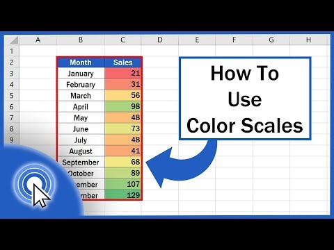
How to Use Color Scales in Excel (Conditional Formatting)
 0:15:42
Conditional formatting EXCEL charts - Dynamic and Automatic Highlighting
Комментарии