Excel - use Max and Large Function with Conditional Formatting by Chris Menard

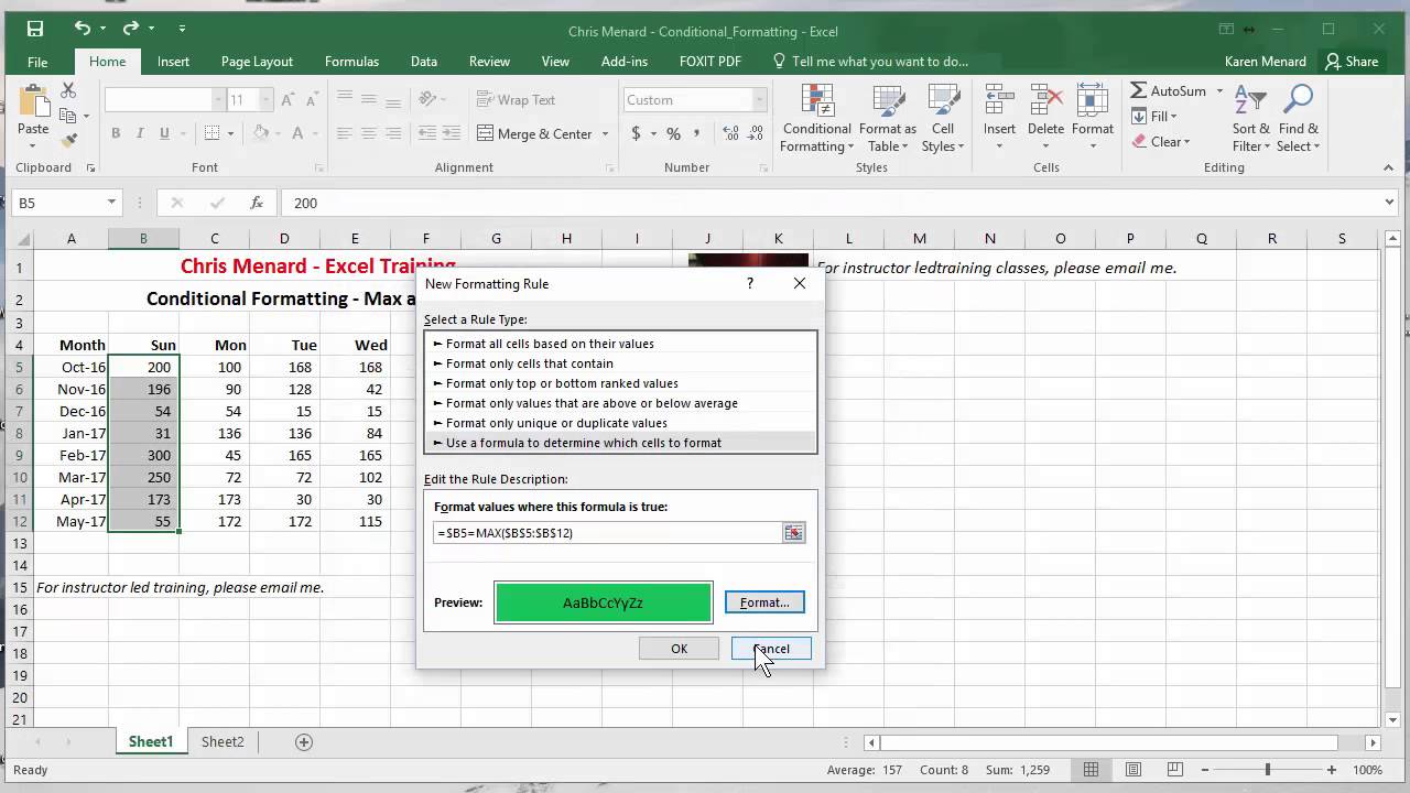
Use Excel's Max and Large Function with Conditional Formatting. If you want to see the highest value in one color and the 2nd highest in another, the max and large functions with conditional formatting will handle that.

Steps:
1. Select your range. My example is B5:B12.
2. Click on Conditional Formatting in Styles Group on the Home Tab.
3. Click New Rule.
4. Select "Use a formula to determine which cells to format".
5. For the highest value, use "=$B5=MAX($B$5:$B$12)" without the quotations.
6. Click on Format and select a Fill color.
7. Click on OK twice.
8. Do the same steps for the 2nd highest which is the Large function. "=$B5=LARGE($B$5:$B$12,2)"

And make sure you subscribe to my channel!

-- EQUIPMENT USED ---------------------------------

-- SOFTWARE USED ---------------------------------

DISCLAIMER: Links included in this description might be affiliate links. If you purchase a product or service with the links I provide, I may receive a small commission. There is no additional charge to you! Thank you for supporting my channel, so I can continue to provide you with free content each week!

[chrismcconnell]

Hey Chris. Great video. Easy to understand and just what i needed. Thanks

[manishagupta]

thank u so so much sir. this is really helpful for me

[pauldavidstewart]

This was great. But what if I want to find the 2nd highest horizontally and not vertically? Like the 2nd highest of the days of the week in row 5? Specifically F5 to H5? When I adjusted your vertical formula to go horizontal it didn't work (but it did vertically like in column B of your example).

[jocelynngh]

when you click on B5 after you put in a new formatting rule, the formula is automatically populated? I am referring to 1:17 to 1:22. Also, how did "Paste" come about?