Google Sheets | SORTN Function | SORT Data & Display Specific No. of Rows | Example | Spreadsheet

Use the Google Sheets SORTN function to sort data and get only the first n rows of a range. Here n is the number of specified rows. SORTN is in contrast to SORT in that the latter sorts and returns all the rows.

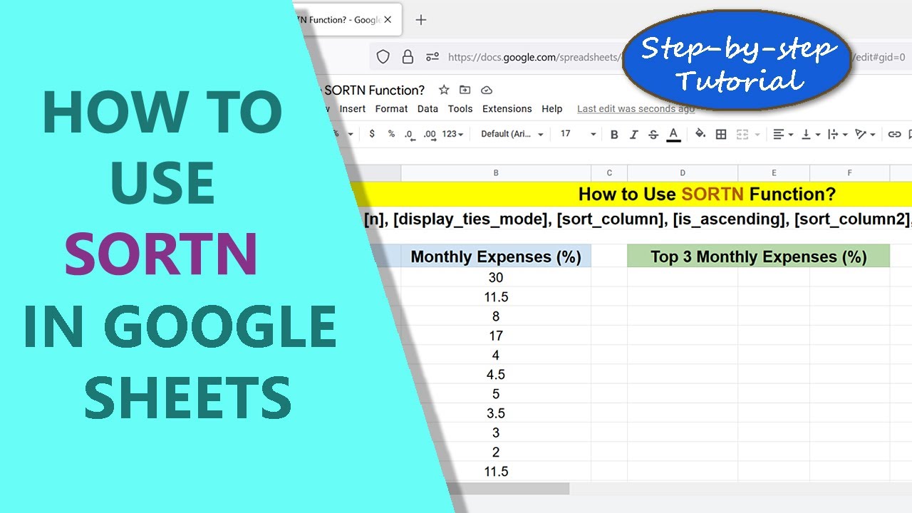
Here is an example of where using the SORTN function would be ideal: Say you have a spreadsheet with two columns, relating to the average monthly expenses. The first column has items like Rent, Groceries, and Insurance, and the second has expenses, represented as the percentage of total income.

If you wish to know, say only the top five expenses, then using SORTN would be a good choice.

-------------------------------------
How to Use SORT in Google Sheets?

Sort the data in an ascending or a descending order using the SORT function. The link to the step-by-step tutorial on SORT is:

-------------------------------------
How to Use TRIM in Google Sheets?

Remove leading or trailing spaces or remove spaces between text using the
TRIM function. Here is the link to the step-by-step video tutorial:

-------------------------------------
How to Use LEN in Google Sheets?

Use the LEN function to calculate the length of a string. The link to the
step-by-step video tutorial on LEN function is:

-------------------------------------
How To Create a Fixed Deposit (FD) Maturity Amount Calculator in Google Sheets?

Here's the link to the step-by-step video tutorial on creating the calculator:

-------------------------------------

Let's look at the format of the SORTN function formula:

=SORTN(range, [n], [display_ties_mode], [sort_column], [is_ascending], [sort_column2], [is_ascending2], […])

Start the formula with an equal-to symbol.

SORTN is the name of the function.

Range is the spreadsheet area with the data to be sorted.

n is optional, and is the number of rows, which are sorted, to return.

display_ties_mode is optional, and is the number that specifies which rows to display.
This argument can have a value of 0, 1, 2, or 3.
0 specifies that a maximum of n rows should be displayed.
1 specifies that a maximum of n rows should be displayed and additional rows that match the nth row, if any.
2 specifies that a maximum of n rows should be displayed after removing any duplicate rows.
3 specifies that a maximum of n rows should be displayed, including any duplicate rows.

sort_column is optional, and is the column by which to sort the data.

is_ascending is optional, and if TRUE the data in the first column is sorted in an ascending order.

sort_column2 is optional, and is the additional sort column.

is_ascending2 is optional, and if TRUE the data in the second sort column is sorted in an ascending order.

NOTE: If n is specified, then display_ties_mode must be specified. If sort_column is specified, is_ascending must be specified, and so on.

Example 1:

=SORTN(A3:B13,5,0,B3:B13,0)

In the SORTN formula:

A3:B13 is the range.

5 specifies the maximum number of rows to be displayed.

0 specifies that maximum n rows (which is 5) should be displayed.

B3:B13 is the range of data by which to sort the same.

0 specifies that the data should be sorted in a descending order.

Example 2:

=SORTN(A3:B13,5,1,B3:B13,0)

The only change in this example, in comparison to the first example, is the value of display_ties_mode argument. This value is 1 in this example. The value specifies that the first five rows should be displayed and any additional rows same as the fifth row.

Take a look at this video tutorial, which gives the steps to use the Google Sheets SORTN function with examples.