What Does It Mean to Solve the Heat Equation PDE? An Introduction with Example Solutions and Graphs

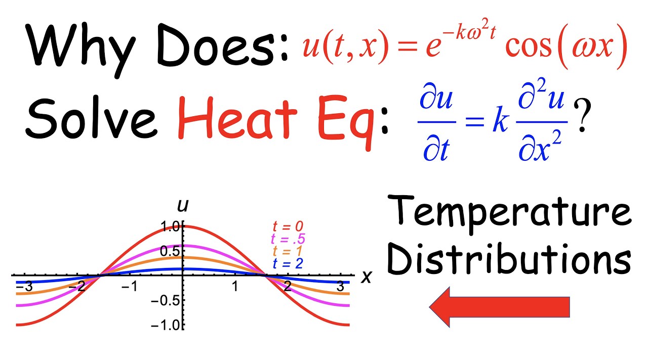
The heat equation partial differential equation (PDE) and its solutions were studied by Joseph Fourier in the early 1800's. But what does it mean for a function (temperature profile) u(t,x) to solve the heat equation? And what does the solution represent? It means that the first partial derivative of u(t,x) with respect to time t is equal to a positive constant multiple of the second partial derivative of u(t,x) with respect to position x (along a finite or infinite "thin rod"). Boundary conditions for the heat equation must also be satisfied: 1) there is an initial temperature profile when t = 0 ("initial data") and, if the thin rod is finite, 2) there are boundary conditions (boundary values) at the endpoints x = a and x = b. These can be fixed value boundary conditions or fixed derivative boundary conditions, for instance. Two example solutions of the heat equation are shown both symbolically and graphically. The first is a cosine (sinusoidal) wave with an exponentially decaying amplitude. The second results from a point "mass" heat source (of "infinity") at x = 0 when t = 0 which decays in a way that its graph always looks like a normal distribution with an increasing variance as time t increases. Calculations are confirmed and animations are made in Mathematica using Manipulate.

Bill Kinney's Differential Equations and Linear Algebra Course, Lecture 35C.

(a.k.a. Differential Equations with Linear Algebra, Lecture 35C, a.k.a. Continuous and Discrete Dynamical Systems, Lecture 35C).

#partialdifferentialequations #heatequation #differentialequations

(0:00) Lecture plans
(1:10) Joseph Fourier was trying to model heat conduction with partial differential equations
(1:54) Finite thin rod case
(2:34) Meaning of variables x (position) and t (time) and u = u(t,x) (temperature)
(5:51) The Heat Equation
(8:53) Want to match initial data and boundary conditions
(10:42) Solutions which are sinusoidal waves whose amplitudes exponentially decrease over time
(15:35) Solutions which are "delta-like" functions which exponentially decay over time
(17:46) Superposition: linear combinations of solutions are solutions
(20:05) Example linear combination of solutions
(21:34) Mathematica calculations and graphs

AMAZON ASSOCIATE
As an Amazon Associate I earn from qualifying purchases.

[georgesadler]

Professor Kinney, thank you for the basic introduction of the Heat Equation Patrial Differential Equation and its nontrivial solutions. I took a senior level course in Partial Differential Equations at the University of Maryland College Park, and this was one of the first topic that was taught in the class. I am familiar with the Heat Equation and its impact on Advanced Mathematics. Linear Systems/Combinations are all tied into the classic Heat Equation.

[nickbe]

Very interesting. I have a question concerning 20:29 when you show the linear combination of the solutions: the cosines with high value of omega are the first who decay after a certain amount of time when you plot the solution? Also another question: does the heat solution have to decay always to zero after a t->infinity in every pde problem? Thanks you a lot!