filmov
tv
Introduction To Optimization: Gradient Based Algorithms

Показать описание
A conceptual overview of gradient based optimization algorithms.
NOTE: Slope equation is mistyped at 2:20, should be delta_y/delta_x.
This video is part of an introductory optimization series.
TRANSCRIPT:
Hello, and welcome to Introduction To Optimization. This video covers gradient based algorithms.
Gradient based algorithms and gradient free algorithms are the two main types of methods for solving optimization problems. In this video, we will learn the basic ideas behind how gradient based solvers work.
Gradient based solvers use derivatives to find the optimum value of a function.
To understand how this works, imagine that you are hiking on a mountainside, trying to find your way to a campsite at the bottom of the mountain. How would you know where to go? Perhaps you could follow a trail, look at a map, or use a GPS. You might even be able to see your destination, and head straight there. Now imagine that you have no map, no GPS, no trail, and there are trees all around that keep you from seeing anything but the area immediately around you. Now what?
Knowing nothing except for the fact that the campsite is at the bottom of the mountain, one possible option is to head downhill. You could look around, evaluate the slope of the mountain in the small area you can see, and walk in the direction with the steepest downhill slope. You could continue doing this, pausing once in awhile to find the best path forward, and eventually make it to the campsite.
On a basic level, this is the same thing that gradient based algorithms do. There are three main steps:
Search Direction: The first step is to pick a direction to go. The solver evaluates the slope by taking the derivative at its current location. In one dimension this derivative is the slope. In more than one dimension, this is called the gradient. The solver then uses this information together with other rules to pick a direction to go. This is called the search direction.
Step Size: The next step is to decide how far to go in the chosen direction. You don’t want to go too far in one direction, or you might end up going back up a different mountain. However, you do want to go far enough to make some progress towards your goal. The value the solver chooses is called the step size.
Convergence Check: Once a direction and a step size are chosen, the solver moves in the chosen direction. Then it checks to see if it has reached the bottom. If not, it uses the slope again to pick a new direction and step size. This continues until the solver reaches the bottom of the mountain, or the minimum. We call this convergence.
There are many variations on the way that these steps are performed, but these are the basic ideas behind how a gradient based optimization algorithm works.
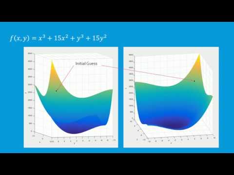
Let’s take a look at what this might look like on an actual function. We’ll try to find the minimum of the equation x^3 + 15x^2 + y^3 +15y^2.
We’ll start out by visualizing the function. This is a plot of the function values over a range from -10 to 10 in both directions. Notice how the function slopes down towards a minimum in the center. To begin, we’ll need to give the optimizer an initial guess. Let’s choose (8,8). Another way we can represent this information is with a contour plot, where the lines represent constant levels or function values.
We can watch now as the optimizer chooses a search direction, and takes a step, a direction, and a step. Eventually it reaches the minimum point at x = 0, y = 0.
Gradient based algorithms have their own strengths and weaknesses. They are widely used, have fast performance, and scale well to large problems. However, they do require smooth, continuous function gradients, and computing those gradients can be computationally expensive. Many gradient based optimizers are also susceptible to finding local minima rather than a global optimum, meaning that they will find the bottom of the closest valley, rather than the lowest point on the whole map. Gradient based optimizers are a powerful tool, but as with any optimization problem, it takes experience and practice to know which method is the right one to use in your situation.
Комментарии
 0:11:04
 0:30:22
 0:27:39
 0:05:25
 0:03:53
 0:11:55
 0:03:06
 0:23:54
 0:27:48
 0:31:59
 1:27:37
 0:15:39
 0:32:22
 0:03:52
 0:07:05
 0:04:14
 0:20:33
 0:22:54
![[DL] Gradient-based optimization:](https://i.ytimg.com/vi/3BCrKkqyuAs/hqdefault.jpg) 0:05:13
0:05:13
 0:10:52
 0:10:01
 0:14:30
 0:17:50