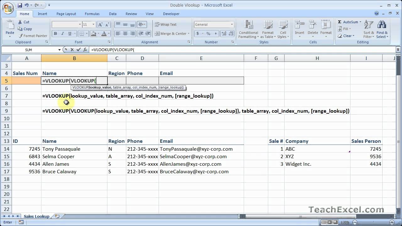
Double Vlookup in Excel - Use Multiple Vlookups Together - Nested Vlookups

Learn how to combine two vlookups into one vlookup function in Excel. This also includes an explanation and example of when or why you would want or need to do this in Excel. Basically, this is just nesting vlookup functions within each other and it will allow you to create more robust and useful formulas in Excel.

This will help you to search through multiple tables at once in Excel in order to get the data that you need. As such, this is one way of creating more useful, albeit complex, Excel spreadsheets and this will help you sift through your data in Excel.

[dyonishosim]

these must be the best Excel tutorials on YT.  Thumbs Up if you agree.
Expertly explained.  Hats off to you sir!!

[granand]

Now we can do the same using power query by joining two tables & merging ..but this is like driving vehicles with gear ..needs genius like this awesome tutor to make me understand

[quambomb]

one of the better tutorials on youtube

[lesliehoward]

Complex and awesome at the same time. Great explanation!

[semperdiscendum]

Thank you for this great video! Please keep teaching us!

[veejay]

greatly expalined..u made it so simple
..thanx

[kirov]

Awesome! Helpful to learn quickly double nested function use. Thank you for your time.

[veenarautela]

Wow...this is what I was looking for 👌

[workonyourbiznotinit]

This is way too cool ! Mr.ExcelGuru ! Appreciate !!

[LearnYouAndMe]

for those who are not comfortable in writing complex or nested formula directly, here is a simple strategy, write helper column or cells then merge formula of a cell in a formula which referring that cell. Example In cell "K1" our final vlookup =VLOOKUP(J1, $A$1:$B$7, 2, FALSE) formula is present, which reference value of helper cell "J1" having vlookup =VLOOKUP(I1, $P$1:$Q$8, 2, FALSE). Now we want to eliminate use of helper cell "J1", so just replace J1 present in "k1" cell formula with VLOOKUP(I1, $P$1:$Q$8, 2, FALSE) [J1 cell vlookup formula]. Now in cell "K1" our formula will becomes =VLOOKUP(VLOOKUP(I1, $P$1:$Q$8, 2, FALSE), $A$1:$B$7, 1, FALSE) after this we can delete helper cell or column.

[cansucelebi]

Thanks :) It's very useful. you save my time

[waterbear]

This method is great, however, I prefer if i can drag the formula down and across then fetch everything as long as it conforms with the criteria. help pls. ty

[angeladevous]

Hi, I have been searching through excel for help with a nested if and vlookup function and haven't been successful.  I was hoping you could help.  I have a table that I must use a nested if and vlookup formula in order to get my results using both vertical and horizontal cells.  I understand nested if formula and vlookup formulas but not able to get them to work together in the same formula using both horizontal and vertical cells.  Any suggestions?

[unboxingreviewvlog]

How use the Vlookup Function in first case and when we drap it to the right it should give the output for all the columns and rows respectively?
*Without disturbing the original data.

[dyonishosim]

hmmm...felt like i just watched Inception all over again. :)

[shau]

Thanks for a nice tutorial. But I have 2 problem:
1`) I have been struggling to design 1 formula for calculating fixed account interests for 4 banks which have different percentages of interest rates for different amounts of money deposited for different times of maturity. Kindly please help me out.

I used nested if but the formula became too long and hence cumbersome and erroneous. I then tried VLOOKUP but it did not work well. Thanks.
2) Is indirect function a lookup function? I tried to use indirect function replacing vlookup, in for example finding number of items sold by one store out of 4 stores in four different cities. It worked with three upper rows but returned error in the last raw. but VLookup worked nicely. Kindly please help. thanks

[greatazmat]

is it possible get result with two to three lookup values and column not confirm?

[jgbalboa]

Or to make an easier example, type two lookups; one that looks for "sales #" and one to look for the "ID." Then "cut" and "sales person" formula and paste it within the "ID" formula place of A5 of the "sales" formula . . . I think.

[oliviermanbode]

interesting, but if you insert an additional column for sales No in your first table, then only 1 vlookup is necessary

[jjj]

How do we use double vlookup with aggregate and search to get multiple results? E.g search Michael and get multiple Michael's.

Thanks