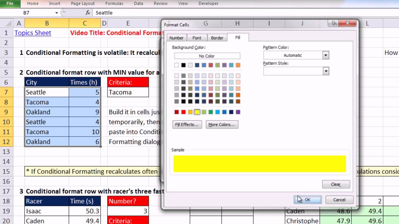
Ctrl + Shift + Enter: Excel Array Formulas 21: Conditional Formatting with Array Formulas

EXCEL ARRAY FORMULAS WORK THE SAME IN ANY VERSION OF EXCEL!!!

This video covers:
1. (00:32 min) Conditional Formatting is volatile: It recalculates often and can slows overall spreadsheet calculation time.
2. (01:07 min) Conditional format row with MIN value for a given city.
3. (08:21 min) Conditional format row with racer's three fastest times using helper cell.

THIS VIDEO SERIES AT YOUTUBE IS THE SAME AS THE DVD FROM EXCELISFUN. THESE VIDEOS ARE BEING GIVEN AWAY FOR FREE AT YOUTUBE. SUPPORT THE CAUSE BY GOING TO AMAZON AND BUYING THE BOOK.
EXCEL ARRAY FORMULAS WORK THE SAME IN ANY VERSION OF EXCEL!!!
Ctrl+Shift+Enter: A Book About Building Efficient Formulas, Advanced Formulas, and Array Formulas for Data Analysis and Calculating Problems
Designed with Excel gurus in mind, this handbook outlines how to create formulas that can be used to solve everyday problems with a series of data values that standard Excel formulas cannot or would be too arduous to attempt. Beginning with an introduction to array formulas, this manual examines topics such as how they differ from ordinary formulas, the benefits and drawbacks of their use, functions that can and cannot handle array calculations, and array constants and functions. Among the practical applications surveyed include how to extract data from tables and unique lists, how to get results that match any criteria, and how to utilize various methods for unique counts. This book contains 529 screen shots.

[excelisfun]

Ctrl + Shift + Enter: Excel Array Formulas 21: Conditional Formatting with Array Formulas 
Download Excel file link below this video.
There are 26 videos in this playlist series.
This video is the same as the video on the DVD, but it is being given away for free here at YouTube.
To Support the cause, go to Amazon and buy the book or DVD. Title is: Ctrl + Shift + Enter: Mastering Excel Array Formulas.
Excel Array Formulas work the SAME in any version of Excel!!!

[ikebana]

Many thanks for your usefull videos^^. You lift me up!!

[qaisarc]

Thank you so much! This was very helpful.

[JamieLHa]

Not related to Excel but could you let me know what software you use to video? I plan to do some tutorial videos and really like what you use now. Thanks.

[ggi]

This is a very good video, thanks. Unfortunately, though, I still cannot get my conditional formula to work in the one sheet that I need it to work. Something like out of the twilight zone is causing it to fail to do what it is supposed to do in that sheet. It's not giving me any errors. It is just not applying tge formatting. Weirdy, when I do the exact same thing in another sheet using the exact same table values and the same conditional formatting formula that I created using INDIRECT, the thing works like a baby. No headaches whatsoever. Why is it not working in the main sheet where I need it to work is beyond comprehension. I checked and double checked everything but there is nothing to explain why it is not applying tge formatting.

Here is the conditional formula that I have for if anyone has any ideas that would be so kind to share with me:

Apply range is C6:P23 in the table with the formatting.

Format cells if:
=COUNTIF(INDIRECT("Default Picks!$C$6:$P$23"), C6)=0

Formatting --> Set to bold text if the values are not the same.

Basically, I have two twin tables placed in different sheets of tge same workbook on Google Sheets. One named Default Picks (populated with text values in the cells). The other, where the conditional formatting is located, is called Revised Picks. The two tables are the same size but in the Revised table cells the values are pulled from other sources and crunched with an array equation. Some of the values from Default Picks remain unchanged while others do change. But this is all irrelevant, really. The point is that I want the values that have changed to be in bold. That is all.

The Indirect in the cond formatting function cross-references the array text values from the Default table (I use INDIRECT because it's in another sheet) and those are matched cell by cell with the corresponding values in the Revised table where the conditional formatting is setup. I only want the values that don't match to appear in bold for better visualization. I get no errors but it just doesn't apply the formatting. And when I test the same elsewhere it works. Why not in that sheet? I'm baffled and frankly out of solutions or things to try. Seems like a simple problem that has turned into a headache. Could this be like a Google Sheets glitch or something? Maybe a corrupted sheet that acts weird.