filmov
tv
Lecture 13: Randomized Matrix Multiplication

Показать описание
MIT 18.065 Matrix Methods in Data Analysis, Signal Processing, and Machine Learning, Spring 2018
Instructor: Gilbert Strang
This lecture focuses on randomized linear algebra, specifically on randomized matrix multiplication. This process is useful when working with very large matrices. Professor Strang introduces and describes the basic steps of randomized computations.
License: Creative Commons BY-NC-SA
 0:52:24
Lecture 13: Randomized Matrix Multiplication
 0:18:46
Sec 2.1 rec matrix multiplication
 1:21:14
Lecture 13 - Matrix operations (IV) & Midterm review (W7D2)
 0:59:10
Lecture 13: Fundamental Matrix
 0:26:28
Introduction to Probability - Verifying Matrix Multipilication
 1:15:06
Lecture 13: Linear Algebra ii
 0:30:05
Implementing Randomized Matrix Algorithms in Parallel and Distributed Environments, Michael Mahoney
 1:21:14
Lecture 13 - Matrix operations IV & Midterm review - W7D2
 0:31:52
Math 350 - Lecture 13 - More advanced matrix manipulation
 1:13:24
Lecture 13, Tutorial 5: Matrix Factorisation, Movie Recommendation
 0:59:17
Matrices - Lecture 13 - Levy-Desplanques theorem, equivalence of matrix norms, errors in inverses
 0:59:52
Scientific Computing Lecture 13: Linear Algebra with BLAS and LAPACK
 0:21:46
MAT 140 Lesson 7: Matrix Multiplication
 0:01:01
ADSP - 13 Matched Filters - 03 Maximizing SNR as Matrix Multiplication
 0:20:25
Introduction to Probability - Verifying Matrix Multipilication
 1:00:27
ARTIFICIAL INTELLIGENCE LECTURE 13
 0:31:33
Randomized Algorithms in Linear Algebra
 0:07:58
Matrix Multiplication | Array In C Programming Part 10
 1:31:30
Lecture 13 - Fundamental Matrix - 2014
 0:57:30
AI4OPT Tutorial Lectures: Randomized Matrix Computations (Part II)
 0:33:26
An Introduction to Randomized Algorithms for Matrix Computations Part 1
 0:23:40
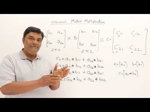
2.9 Strassens Matrix Multiplication
 0:23:52
ARM Lecture 13 Programming LCD with Matrix Keypad Interface
 1:17:03
EfficientML.ai Lecture 13 - Transformer and LLM (Part II) (MIT 6.5940, Fall 2023, Zoom)
Комментарии