How to Use the IFERROR Function in Excel | Using IFERROR in Excel Formula

In this video, we will teach you how to use the IF ERROR function in Excel.

This function enables you to return a specific value if there is an error in the calculation. This way we can handle errors in our calculation.

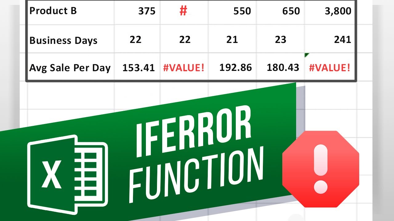
If you look at the sales forecast sheet here, you can see that there are a number of error values in the data. Notice that the SUM function in the total over here overlooks these values by default. But, if we were to calculate average sale per day, you can see that a few totals here are returning error values, and therefore the entire total value here will return an error as well.

For calculating average sales per day, we have simply added sales for both products and divided by the number of working days. For eliminating errors here, we will have to slightly tweak the formula.

In the formula bar, after the “equals to” sign, let’s type IF ERROR and make sure the entire calculation is separated within brackets, like so. You can see that the entire original formula used for the calculation is within the red brackets. Next, let’s enter a comma and type ZERO in inverted commas. What we’re basically saying is that if this calculation returns an error, the return value should be ZERO.

Let’s copy and paste the same formula to the rest of the cells. Over here, you can see that for those months the formula returns an error, ZERO value is displayed in average sales per day, without effecting the total here.

Now instead of ZERO, you can even leave the cell blank. This way at-least you can get the total value here while easily spotting and correcting the data so that it can be added in the total.

That’s all!

❓💬 Is there any excel function you would like to know more about? Let us know in the comments below.

#HowTech #Excel
--------------------------------------------------------------------------------------------------------------